1. Chapter 9 Recursion © 2006 Pearson Education Inc., Upper Saddle River, NJ. All rights reserved.

2. Overview ● 9.1 – Introduce the recursive way of thinking. ● 9.2 – Recursive algorithms requires new techniques. ● 9.3 and 9.4 – Recursive sorting algorithms are introduced. ● 9.5 – Converting recursive algorithms into a nonrecursive form.

3. Computing Factorial 0! = factorial(0) = 1; // factorial is a method n! = factorial(n) = n*factorial(n-1); 3! = 3 * 2 *1 = 6 factorial(3) = 3 * factorial(2) = 3 * (2 * factorial(1)) = 3 * ( 2 * (1 * factorial(0))) = 3 * ( 2 * ( 1 * 1))) = 3 * ( 2 * 1) = 3 * 2 = 6

4. Computing Factorial (recursive) 1. import javax.swing.JOptionPane; 2. public class ComputeFactorial { 3. /** Main method */ 4. public static void main(String[] args) { 5. // Prompt the user to enter an integer 6. String intString = JOptionPane.showInputDialog( 7. "Please enter a non-negative integer:"); 8. // Convert string into integer 9. int n = Integer.parseInt(intString); 10. // Display factorial 11. JOptionPane.showMessageDialog(null, 12. "Factorial of " + n + " is " + factorial(n)); 13. }

5. Computing Factorial (recursive) 1. /** Return the factorial for a specified index */ 2. static long factorial(int n) { 3. if (n == 0) // Stopping condition 4. return 1; // factorial(0) = 1 5. else// Call factorial recursively // factorial(n) = n*factorial(n-1); 6. return n * factorial(n - 1); 7. } 8. }

6. Computing Factorial factorial(3) animation factorial(0) = 1; factorial(n) = n*factorial(n-1);

7. Computing Factorial factorial(3) = 3 * factorial(2) animation factorial(0) = 1; factorial(n) = n*factorial(n-1);

8. Computing Factorial factorial(3) = 3 * factorial(2) = 3 * (2 * factorial(1)) animation factorial(0) = 1; factorial(n) = n*factorial(n-1);

9. Computing Factorial factorial(3) = 3 * factorial(2) = 3 * (2 * factorial(1)) = 3 * ( 2 * (1 * factorial(0))) animation factorial(0) = 1; factorial(n) = n*factorial(n-1);

10. Computing Factorial factorial(3) = 3 * factorial(2) = 3 * (2 * factorial(1)) = 3 * ( 2 * (1 * factorial(0))) = 3 * ( 2 * ( 1 * 1))) animation factorial(0) = 1; factorial(n) = n*factorial(n-1);

11. Computing Factorial factorial(3) = 3 * factorial(2) = 3 * (2 * factorial(1)) = 3 * ( 2 * (1 * factorial(0))) = 3 * ( 2 * ( 1 * 1))) = 3 * ( 2 * 1) animation factorial(0) = 1; factorial(n) = n*factorial(n-1);

12. Computing Factorial factorial(3) = 3 * factorial(2) = 3 * (2 * factorial(1)) = 3 * ( 2 * (1 * factorial(0))) = 3 * ( 2 * ( 1 * 1))) = 3 * ( 2 * 1) = 3 * 2 animation factorial(0) = 1; factorial(n) = n*factorial(n-1);

13. Computing Factorial factorial(3) = 3 * factorial(2) = 3 * (2 * factorial(1)) = 3 * ( 2 * (1 * factorial(0))) = 3 * ( 2 * ( 1 * 1))) = 3 * ( 2 * 1) = 3 * 2 = 6 animation factorial(0) = 1; factorial(n) = n*factorial(n-1);

14. Trace Recursive factorial animation Executes factorial(4)

15. Trace Recursive factorial animation Executes factorial(3)

16. Trace Recursive factorial animation Executes factorial(2)

17. Trace Recursive factorial animation Executes factorial(1)

18. Trace Recursive factorial animation Executes factorial(0)

19. Trace Recursive factorial animation returns 1

20. Trace Recursive factorial animation returns factorial(0)

21. Trace Recursive factorial animation returns factorial(1)

22. Trace Recursive factorial animation returns factorial(2)

23. Trace Recursive factorial animation returns factorial(3)

24. Trace Recursive factorial animation returns factorial(4)

25. factorial(4) Stack Trace

26. Other Examples f(0) = 0; f(n) = n + f(n-1); Example: compute f(5) ?

27. Fibonacci Numbers Finonacci series: 0 1 1 2 3 5 8 13 21 34 55 89… indices: 0 1 2 3 4 5 6 7 8 9 10 11 fib(0) = 0; fib(1) = 1; fib(index) = fib(index - 2) + fib(index - 1); for index >=2 fib(3) = fib(1) + fib(2) = fib(1) + (fib(0) + fib(1)) = 1 + 0 + 1 = 2 ComputeFibonacci

28. Fibonnaci Numbers, cont.

29. Characteristics of Recursion ● All recursive methods have the following characteristics: – One or more base cases (the simplest case) are used to stop recursion. – Every recursive call reduces the original problem, bringing it closer to a base case until it becomes that case. ● In general, to solve a problem using recursion, you break it into subproblems. ● If a subproblem resembles the original problem, you can apply the same approach to solve the subproblem recursively. ● This subproblem is almost the same as the original problem in nature with a smaller size.

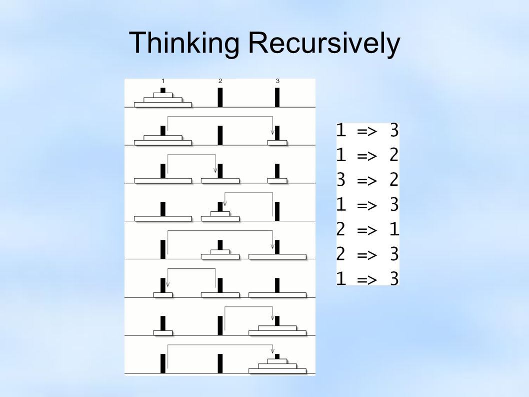
30. Thinking Recursively

32. ● One-disk puzzle is trivial. ● The puzzle for two disks

33. Thinking Recursively ● Method for the three-disk puzzle ● Lines 4 to 6: move the first 2 disks from the source to the spare peg (use the source peg as “source”, dest peg as “spare”, and the spare peg as “dest”). ● Line 8: move the last (bottom) peg from source to dest. ● Lines 10 to 12: move the first 2 disks from the spare peg to the dest peg (use the spare peg as “source”, source peg as “spare” and the dest peg as “dest”).

34. Thinking Recursively ● By invoking hanoi2() we can write a shorter version of hanoi3(). ● Rewrite hanio2() using hanoi1()

35. Thinking Recursively ● We now have a pattern that will allow us to write a method to solve the puzzle for any number of disks. – It would be much better if we could write a single method which would work for any number of disks. ● Recursive method – A method which invokes itself.

36. Thinking Recursively ● Base case – To prevent the recursion from continuing indefinitely – It is the stop condition.

37. Thinking Recursively ● In general, to solve a problem recursively, we have two cases: – The base case, where we can solve the problem directly. – The recursive case, where we solved the problem in terms of easier subproblems. ● Subproblem leads to the base case.

38. Tower of Hanoi (recursive) 1. import javax.swing.JOptionPane; 2. public class TowersOfHanoi { 3. /** Main method */ 4. public static void main(String[] args) { 5. // Read number of disks, n 6. String intString = JOptionPane.showInputDialog(null, 7. "Enter number of disks:"); 8. // Convert string into integer 9. int n = Integer.parseInt(intString); 10. // Find the solution recursively 11. System.out.println("The moves are:"); 12. moveDisks(n, 'A', 'B', 'C'); 13. }

39. Tower of Hanoi (recursive), cont. 1. /** The method for finding the solution to move n disks 2. from fromTower to toTower with auxTower */ 3. public static void moveDisks(int n, char fromTower, 4. char toTower, char auxTower) { 5. if (n == 1) // Stopping condition 6. System.out.println("Move disk " + n + " from " + 7. fromTower + " to " + toTower); 8. else { 9. moveDisks(n - 1, fromTower, auxTower, toTower); 10. System.out.println("Move disk " + n + " from " + 11. fromTower + " to " + toTower); 12. moveDisks(n - 1, auxTower, toTower, fromTower); 13. } 14. } 15. }

40. Thinking Recursively ● Printing a LinkedList backward. (a, b, c  c, b, a) – Iterative approach (Figure 9-11, p228) ● This method works, but it is not very efficient. – Invokes the get() method each time. – Its time complexity is Θ(n 2 ).

41. Thinking Recursively ● Recursive solution for printing a LinkedList backward: – If there are no nodes, return the empty String. (base case) – Otherwise, generate a String for the rest of the list (the part after the first item). Add the first item to the end of this String and return it.

42. Thinking Recursively ● To show that a recursive algorithm works correctly: – Show that the base case works correctly. – Show that if the recursive method works for a problem of size n – 1, then it works for a problem of size n. ● Base case – ToStringReversed() returns “()”.

43. Thinking Recursively ● Assume that node is a reference to the first of a chain of n nodes

44. Thinking Recursively ● If we assume that the recursive invocation toStringReversedHelper(node.getNext()) correctly returns the String "D C B“ ● then toStringReversedHelper(node.getNext()) + Node.getItem() + " " evaluates to "D C B A ", which is what we want. ● If it works for n-1 nodes, it works for a chain of n nodes.

45. Thinking Recursively ● ToStringReversed() for our ArrayList class. – Again we need a helper method, and the design of the algorithm is similar: ● If there are no elements being considered, return the empty String. ● Otherwise, generate a String for all of the elements after the current one. Add the current element to the end of this String and return it.

46. Thinking Recursively Fig. 9-14: The toStringReversed method for ArrayList class

47. Analyzing Recursive Algorithms ● Analyze a recursive algorithm we must think recursively, in terms of a base case and a recursive case. – toStringReversedHleper() — a recurrence. ● Solving a recurrence means transforming it with T(n) on the left and no mention of T (make T disappear) on the right.

48. Analyzing Recursive Algorithms ● The base must work exactly to constitute a solution. – Guessing T(n) = n + 1 – ToStringReversed() runs in linear time. – Its time complexity is Θ(n). – It is much better than the iterative approach Θ(n 2 ).

49. Analyzing Recursive Algorithms ● The recurrence for hanoi():

50. Analyzing Recursive Algorithms ● This expansion continues until we have many copies of T(1). ● There are n levels, corresponding to T(n) down through T(1). ● Therefore the bottommost level is level n-1.

51. Analyzing Recursive Algorithms ● Total number of steps: (p234) ● Verification that the solution is correct. ● Solved! We conclude that hanoi() takes time in Θ(2 n ).

52. Analyzing Recursive Algorithms ● The recursion tree method can be used to analyze algorithms with only one recursive call. – Example: Assuming n is even:

53. Merge Sort ● The recursive idea behind merge sort is: – If there is only one number to sort, do nothing. – Otherwise, divide the numbers into two groups. – After divided, if data size is odd, then the left group will be one larger than the second group. For example, if there are 9 integers to be sorted, then the left group will have 5 numbers and the right group will have 4 numbers after divided. – Recursively sort each group, then merge the two sorted groups into a single sorted array.

54. Merge Sort

55. Merge Sort Example 38617254 72543861 38617254 38617245 1638 ============================ Merge Steps ========================= ============================= Split Steps ========================== 4527 13682457 12345678

56. Merge Sort ● Merge sort is an example of a divide-and- conquer algorithm. ● A sorting algorithm that modifies an existing array, such as insertion sort, is called an in- place sort (sort inside the array). ● Merge sort is not an in-place sort.

57. Merge Sort

58. ● The merge() method combines two sorted arrays into one longer sorted array.

59. Merge Sort ● merge() method takes linear time in the total length of the resulting array.

60. Merge Sort ● mergeSortHelper recurrence.

61. Quicksort ● Another divide-and-conquer sorting algorithm. ● Here's the plan: – If there are zero or one number to sort, do nothing. – Otherwise, partition the region into “small” and Large” numbers, moving the small numbers to the left and the large numbers to the right. Recursively sort each section. The entire array is now sorted.

62. Quicksort ● Partitioning algorithm begins by choosing some array element as the pivot. ● Usually choose the rightmost element in each partition as the pivot. ● Numbers less than or equal to the pivot are considered small, while numbers greater than the pivot are considered large.

63. Quicksort ● As it runs, the algorithm maintains four regions: – Those numbers known to be small. – Those numbers know to be large. – Those numbers which haven't been examined yet. – The pivot itself. ● The four regions: – data[bottom] through data[firstAfterSmall - 1] are known to be small. – data[firstAfterSmall] through data[i-1] are known to be large. – data[i] through data[top-1] have not yet been examined. – The pivot is at data[top].

64. Quicksort

65. Quick Sort Example 38617254 76583124 4 56 8 7 31287654 312 132 123 123 765 567 The 8 integers are sorted!

66. Quicksort

68. ● Partition() is linear time ● Best case O(n log n), but partition() might not divide the region evenly in half. ● Worst case:

69. Quicksort ● Quicksort is better than insertion sort, but not as good as merge sort. – Since it has a low constant factor associated with its running time, and operates in place, Quicksort is sometimes used instead of merge sort when n is not expected to be very large.

70. Quicksort ● Class java.util.Arrays has several overloaded versions of the static method sort(). – The ones for arrays of primitive types use an optimized version of Quicksort that makes the worst-case behavior unlikely. – The version for arrays of objects uses merge sort. ● The difference has to do with the fact that two objects that are equals() may not be identical. ● If a sort keeps such elements in the same order as the original array, the sort is said to be stable. ● Merge sort is stable, but Quicksort is not.

71. Avoiding Recursion ● All other things being equal, it is better to avoid recursion. – Every time we invoke a method, we have to push a frame onto the call stack. – This uses both time and memory. – These optimizations may improve efficiency at the expense of program clarity; this trade off is not always worthwhile.

72. Avoiding Recursion ● If we fail to include a base case in a recursive method: java.lang.StackOverflowError – We run out of memory, the stack overflows. ● An iterative program which fails to include a proper stopping condition will simply run forever.

73. Avoiding Recursion ● Tail recursive algorithms are easy to convert to iteration. ● In tail recursive algorithms the recursive invocation is the very last thing we do.

74. Avoiding Recursion ● Instead of recurring with new arguments we simply change the values of the existing arguments and go back to the beginning.

75. Avoiding Recursion ● Using the loop test to handle the base case equivalent.

76. Avoiding Recursion ● If a recursive algorithm is not tail recursive, the only way to convert it into iterative form may be to manage our own version of the call stack. ● This is complicated and, since it does not eliminate stack manipulation, rarely worth the effort. ● Certain non-tail-recursive algorithms can be made far more efficient by converting them into iterative form.

77. Avoiding Recursion ● Fibonacci Sequence: – Begin with a pair of newborn rabbits, one male and one female. – Beginning in its second month of life, each pair produces another pair every month. – Assuming the rabbits never die, how many pairs will there be after n months?

78. Avoiding Recursion ● Woefully inefficient. ● F(n) Θ(Φ n ), where Φ (the lower-case Greek letter phi) is the golden ratio, roughly 1.618. ● Not tail recursive. ● fibo() does a lot of redundant work.

79. Avoiding Recursion

80. Iterative Fibonacci Program // An iterative program to generate the Fibonacci numbers. // Let n = 6. public class IterativeFibonacci { public static void main(String args[]) { int oneBefore=1, twoBefore=0, fiboNum=0; for (int i=2; i<=6; i++) { fiboNum = oneBefore + twoBefore; oneBefore = fiboNum; twoBefore = oneBefore; } System.out.println("The Fibonacci(6) is:" + fiboNum); }

81. Avoiding Recursion ● Dynamic programming – Technique for improving the efficiency of recursive algorithms that do redundant work. – Solutions to subproblems are stored (e.g. in an array) so that they can be looked up rather than recomputed.

82. Summary ● To solve a problem recursively, we define a simple base case and a recursive case. ● Recursive case solves the problems in terms of subproblems which are closer to the base case. ● Recursive algorithms are analyzed using recurrences. – To solve a recurrence, expand it into a recursion tree, then determine the number of steps at each level and the number of levels. – Plug the solution into the recurrence to verify it is correct.

83. Summary ● Merge sort and Quicksort – Both of these are divide-and-conquer algorithms which divide the data into parts, recursively sort the parts, and then recombine the solutions. – Merge sort, the hard work is in the recombining. ● Θ (n log n) – Quicksort, the hard work is in the dividing. ● Θ (n log n) on average, its worst-case running time is quadratic. ● Simple improvements can make the worst case unlikely.

84. Summary ● Recursion allows for the design of powerful, elegant algorithms, but it uses up time and space for the call stack. – Efficiency can sometimes be improved by eliminating recursion. – A tail-recursive algorithm can easily be converted into a loop. – If the algorithm is only returning a value (as opposed to modifying an existing data structure), redundant computation can be avoided by storing the results of previous invocation in a table (array).

85. Chapter 9 Self-Study Homework ● Pages: 231-248 ● Do the following Exercises: 9.1, 9.2, 9.5, 9.6, 9.7, 9.18.