Download presentation
Presentation is loading. Please wait.

1
Temperature correction of energy consumption time series Sumit Rahman, Methodology Advisory Service, Office for National Statistics

2
Final consumption of energy – natural gas Energy consumption depends strongly on air temperature – so it is seasonal

3
Average monthly temperatures But temperatures do not exhibit perfect seasonality

4
Seasonal adjustment in X12-ARIMA Y = C + S + I Series = trend + seasonal + irregular Use moving averages to estimate trend Then use moving averages on the S + I for each month separately to estimate S for each month Repeat two more times to settle on estimates for C and S; I is what remains

5
Seasonal adjustment in X12-ARIMA Y = C × S × I Common for economic series to be modelled using the multiplicative decomposition, so seasonal effects are factors (e.g. “in January the seasonal effect is to add 15% to the trend value, rather than to add £3.2 million”) logY = logC + logS + logI
 logY = logC + logS + logI.")
6
Temperature correction – coal In April 2009 the temperature deviation was 1.8°(celsius) The coal correction factor is 2.1% per degree So we correct the April 2009 consumption figure by 1.8 × 2.1 = 3.7% That is, we increase the consumption by 3.7%, because consumption was understated during a warmer than average April
 The coal correction factor is 2.1% per degree So we correct the April 2009 consumption figure by 1.8 × 2.1 = 3.7% That is, we increase the consumption by 3.7%, because consumption was understated during a warmer than average April")
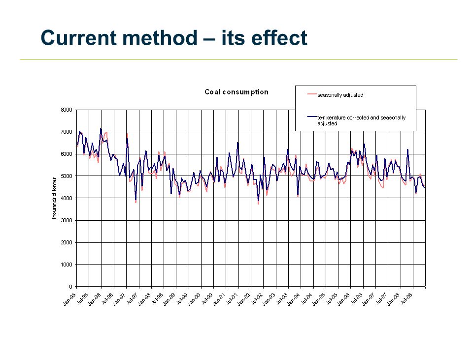
7
Current method – its effect

9
Regression in X12-ARIMA Use x it as explanatory variables (temperature deviation in month t, which is an i-month) 12 variables required In any given month, 11 will be zero and the twelfth equal to the temperature deviation
 12 variables required In any given month, 11 will be zero and the twelfth equal to the temperature deviation")
10
Regression in X12-ARIMA Why won’t the following work?

11
Regression in X12-ARIMA So we use this:

12
Regression in X12-ARIMA More formally, in a common notation for ARIMA time series work: ε t is ‘white noise’: uncorrelated errors with zero mean and identical variances

13
Regression in X12-ARIMA An iterative generalised least squares algorithm fits the model using exact maximum likelihood By fitting an ARIMA model the software can fore- and backcast, and we can fit our linear regression and produce (asymptotic) standard errors
 standard errors")
14
Coal – estimated coefficients

15
Interpreting the coefficients For January the coefficient is -0.044 The corrected value for X12 is The temperature correction is If the temperature deviation in a January is 0.5°, the correction is We adjust the raw temperature up by 2.2% Note the signs!

16
Interpreting the coefficients If is small then So a negative coefficient is interpretable as a temperature correction factor as currently used by DECC Remember: a positive deviation leads to an upwards adjustment

17
Coal – estimated coefficients

18
Gas – estimated coefficients

19
Smoothing the coefficients for coal

20
Comparing seasonal adjustments

21
Heating degree days The difference between the maximum temperature in a day and some target temperature If the temperature in one day is above the target then the degree day measure is zero for that day The choice of target temperature is important

22
Smoothing the coefficients, heating degree days model (Eurostat measure)
")
23
Effect on coal seasonal adjustment

24
The difference temperature correction can make! Primary energy consumption Million tonnes of oil equivalent UnadjustedTemperature adjusted 2009211.1212.6 2010217.3211.3 Annual change+2.9%-0.6%

Similar presentations