Download presentation
Presentation is loading. Please wait.

1
Univariate EDA (Exploratory Data Analysis)
")
4
EDA John Tukey (1970s) data –two components: smooth + rough patterned behaviour + random variation resistant measures/displays –little influenced by changes in a small proportion of the total number of cases –resistant to the effects of outliers –emphasizes smooth over rough components concepts apply to statistics and to graphical methods
 data –two components: smooth + rough patterned behaviour + random variation resistant measures/displays –little influenced by changes in a small proportion of the total number of cases –resistant to the effects of outliers –emphasizes smooth over rough components concepts apply to statistics and to graphical methods")
5
Tree Ring dates (AD) 1255 1239 1162 1239 1240 1243 1241 1241 1271 9 dendrochronology dates what do they mean???? usually helps to sort the data…

6
Stem-and-Leaf Diagram 1162 1239 1239 1240 1241 1241 1243 1255 1271 11|62 12|39,39,40,41,41,43,55,71 original values preserved no rounding, no loss of information…

7
can simplify in various ways… 11|6 12|44444467 –‘leaves’ rounded to nearest decade –‘stem’ based on centuries

8
1162 1239 1239 1240 1241 1241 1243 1255 1271 116|2 117| 118| 119| 120| 121| 122| 123|99 124|0113 125|5 126| 127|1 ‘stem’ based on decades…

9
Stem-and-Leaf Diagram 11|6 12|44444467 –‘leaves’ rounded to nearest decade –‘stem’ based on centuries 1162 1239 1239 1240 1241 1241 1243 1255 1271

10
Stem-and-Leaf Diagram 11|62 12|39,39,40,41,41,43,55,71 original values preserved no rounding, no loss of information…

11
1162 1239 1239 1240 1241 1241 1243 1255 1271 116|2 117| 118| 119| 120| 121| 122| 123|99 124|0113 125|5 126| 127|1 ‘stem’ based on decades…

12
1162 1239 1239 1240 1241 1241 1243 1255 1271 116|2 117| 118| 119| 120| 121| 122| 123|99 124|0113 125|5 126| 127|1 highlights existence of gaps in the distribution of dates, groups of dates…

13
R stem() vu round(runif(25, 0, 50),0); stem(vu) vn round(rnorm(25, 25, 10),0); stem(vn) stem(vn, scale=2)
 vu round(runif(25, 0, 50),0); stem(vu) vn round(rnorm(25, 25, 10),0); stem(vn) stem(vn, scale=2)")
14
unit 1unit 2 12.616.2 11.616.4 16.313.8 13.113.2 12.111.3 26.914 9.79 11.512.5 14.815.6 13.511.2 12.412.2 13.615.5 11.7 926 25 24 23 22 21 20 19 18 17 31624 1556 8140 6511328 6411225 6511237 10 790 unit 1unit 2 Back-to-back stem-and-leaf plot rim diameter data (cm)
")
15
percentiles useful for constructing various kinds of EDA graphics don’t confuse percentile with percent or proportion Note: frequency = count relative frequency = percent or proportion

16
percentiles “the pth percentile of a distribution: number such that approximately p percent of the values in the distribution are equal or less than that number…” can be calculated for numbers that actually exist in the distribution, and interpolated for numbers than don’t…

17
percentiles sort the data so that x 1 is the smallest value, and x n is the largest (where n=total number of cases) x i is the p i th percentile of a dataset of n members where:
 x i is the p i th percentile of a dataset of n members where:")
18
p 1 = 100(1 - 0.5) / 7 = 7.1 p 2 = 100(2 - 0.5) / 7 = 21.4 p 3 = 100(3 - 0.5) / 7 = 35.7 p 4 = 100(4 - 0.5) / 7 = 50 etc… [1]
![p 1 = 100( ) / 7 = 7.1 p 2 = 100( ) / 7 = 21.4 p 3 = 100( ) / 7 = 35.7 p 4 = 100( ) / 7 = 50 etc… [1]](http://images.slideplayer.com/23/6562229/slides/slide_18.jpg "p 1 = 100( ) / 7 = 7.1 p 2 = 100( ) / 7 = 21.4 p 3 = 100( ) / 7 = 35.7 p 4 = 100( ) / 7 = 50 etc… [1]")
19
25 ? 85 ? 50 50 th percentile: i=(7*50)/100 +.5 i=4, x i =7 25 th percentile: i=(7*25)/100 +.5 i=2.25, 3<x i <5
/ i=4, x i =7 25 th percentile: i=(7*25)/ i=2.25, 3<x i <5.")
20
? if i integer, then… k = integer part of i; f = fractional part of i x int = interpolated value of x x int = (1-f)x k + fx k+1 x int = (1-.25)*3+.25*5 x int = 3.5 25 th percentile: i=(7*25)/100 +.5 i=2.25, 3<x i <5 25
x k + fx k+1 x int = (1-.25)*3+.25*5 x int = th percentile: i=(7*25)/ i=2.25, 3<x i <5 25")
21
use R!! test<-c(1,3,5,7,9,9,14) quantile(test,.25, type=5)
 quantile(test,.25, type=5)")
22
75 th 25 th 50 th percentiles: interquartile range (midspread) upper hingelower hinge inner fence “boxplot” (1.5 x midspread)
 upper hingelower hinge inner fence boxplot (1.5 x midspread)")
23
Figure 6.25: Internal diversity of neighbourhoods used to define N-clusters, measured by the 'evenness' statistic H/Hmax on the basis of counts of various A-clusters, and broken down by N-cluster and phase. [Boxes encompass the midspread; lines inside boxes indicate the median, while whiskers show the range of cases that fall within 1.5-times the midspread, above or below the limits of the box.]

24
Cleveland, W. S. (1985) The Elements of Graphing Data.
 The Elements of Graphing Data.")
25
Histograms divide a continuous variable into intervals called ‘bins’ count the number of cases within each bin use bars to reflect counts intervals on the horizontal axis counts on the vertical axis

26
“bins” Histogram counts percent

27
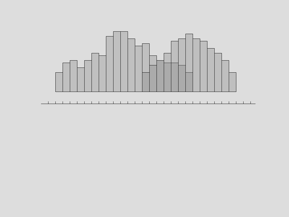
useful for illustrating the shape of the distribution of a batch of numbers may be helpful for identifying modes and modal behaviour Histograms

28
mode mode? mode! the distribution is clearly bimodal may be multimodal…

32
important variables in histogram constuction: bin width bin starting point

33
boundaries of ‘bins’… bins: 1-2; 2-3; 3-4... George Cowgill: construct ‘bins’ of whole multiples of “minimum meaningful measurement units” (“mmmus”) where to count a value like ‘2.0’? Shennan: really means 1.0-1.9; 2.0-2.9; 3.0-3.9... is this OK?? 2.0 = 1.95> <2.05 mmmu=1.95-2.05; 2.05-2.15; 2.15-2.25; 2.25-2.35…
 where to count a value like ‘2.0’. Shennan: really means ; ; is this OK = 1.95> <2.05 mmmu= ; ; ; ….")
34
1.80 - 1.992.00 - 2.19 1.8 - 2.02.0 - 2.2 1.952.05 observed value 2.0… 1.75 - 1.951.95 - 2.15

35
smoothing histograms may want to accentuate the ‘smooth’ in a data distribution… calculate “running averages” on bin counts level of smoothing is arbitrary…

37
histogram / barchart variations 3d stacked dual frequency polygon kernel density methods

38
dual barchart

39
Site 1 Site 2

40
‘mirror’ barchart

41
stacked barchart

42
3d barchart

44
frequency polygon

45
kernel density model

47
controlling kernel density plots… hd <- density(XX) hh <- hist(XX, plot=F) maxD <- max(hd$y) maxH <- max(hh$density) Y <- c(0, max(c(maxD, maxH))) hist(XX, freq=F, ylim=Y) lines(density(XX))
 hh <- hist(XX, plot=F) maxD <- max(hd$y) maxH <- max(hh$density) Y <- c(0, max(c(maxD, maxH))) hist(XX, freq=F, ylim=Y) lines(density(XX))")
48
Dot Plot [R: dotchart()]
![Dot Plot [R: dotchart()]](http://images.slideplayer.com/23/6562229/slides/slide_48.jpg "Dot Plot [R: dotchart()]")
50
Dot Histogram [R: stripchart()] 12345678910 VAR00003 12345678910 VAR00003 12345678910 VAR00003 method = “stack”
![Dot Histogram [R: stripchart()] VAR VAR VAR00003 method = stack](http://images.slideplayer.com/23/6562229/slides/slide_50.jpg "Dot Histogram [R: stripchart()] VAR VAR VAR00003 method = stack")
51
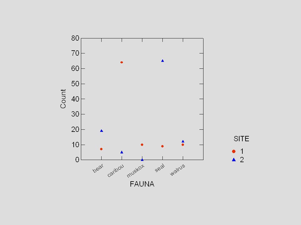
cooking/serviceserviceritual line plot

52
cooking/serviceserviceritual

54
20% 19% 18% 21% 22% pie chart

56
10 20 30 40 50 60 70 80 90 100 percent 10 20 30 40 50 60 70 80 90 100 cumulative percent Cumulative Percent Graph

57
10 20 30 40 50 60 70 80 90 100 cumulative percent some useful statistical measures (ordinal or ratio scale) can be misleading when used with nominal data good for comparing data sets Cumulative Percent Graph
 can be misleading when used with nominal data good for comparing data sets Cumulative Percent Graph")
Similar presentations


 2004 Brooks/Cole, a division of Thomson Learning, Inc. Chapter Two Treatment of Data.>")

>")


