1. Face Recognition and Feature Subspaces
11/07/13
Chuck Close, self portrait
Lucas by Chuck Close
Devi Parikh
Virginia Tech
Slides borrowed from Derek Hoiem, who borrowed some slides from Lana Lazebnik, Silvio Savarese, Fei-Fei Li

2. This class: face recognition
Two methods: “Eigenfaces” and “Fisherfaces”
Feature subspaces: PCA and FLD
Look at results from recent vendor test
Look at interesting findings about human face recognition

3. Applications of Face Recognition
Surveillance

4. Applications of Face Recognition
Album organization: iPhoto 2009

5. Facebook friend-tagging with auto-suggest

6. Face recognition: once you’ve detected and cropped a face, try to recognize it
Detection
Recognition
“Sally”

7. Face recognition: overview
Typical scenario: few examples per face, identify or verify test example
What’s hard: changes in expression, lighting, age, occlusion, viewpoint
Basic approaches (all nearest neighbor)
Project into a new subspace (or kernel space) (e.g., “Eigenfaces”=PCA)
Measure face features
Make 3d face model, compare shape+appearance (e.g., AAM)

8. Typical face recognition scenarios
Verification: a person is claiming a particular identity; verify whether that is true
E.g., security
Closed-world identification: assign a face to one person from among a known set
General identification: assign a face to a known person or to “unknown”

9. What makes face recognition hard?
Expression

10. What makes face recognition hard?
Lighting

11. What makes face recognition hard?
Occlusion

12. What makes face recognition hard?
Viewpoint

13. Simple idea for face recognition
Treat face image as a vector of intensities
Recognize face by nearest neighbor in database

14. The space of all face images
When viewed as vectors of pixel values, face images are extremely high-dimensional
100x100 image = 10,000 dimensions
Slow and lots of storage
But very few 10,000-dimensional vectors are valid face images
We want to effectively model the subspace of face images

15. The space of all face images
Eigenface idea: construct a low-dimensional linear subspace that best explains the variation in the set of face images

16. Principal Component Analysis (PCA)
Given: N data points x1, … ,xN in Rd
We want to find a new set of features that are linear combinations of original ones: u(xi) = uT(xi – µ) (µ: mean of data points)
Choose unit vector u in Rd that captures the most data variance
Forsyth & Ponce, Sec ,

17. Principal Component Analysis
Direction that maximizes the variance of the projected data: N
Maximize
subject to ||u||=1
Projection of data point N
1/N
Covariance matrix of data = XXT
The direction that maximizes the variance is the eigenvector associated with the largest eigenvalue of Σ

18. Implementation issue Covariance matrix is huge (M2 for M pixels)
But typically # examples << M
Simple trick
X is MxN matrix of normalized training data
Solve for eigenvectors u of XTX instead of XXT
XTXu = lu
XXTXu = lXu
(XXT)Xu = l(Xu).
Then Xu is eigenvector of covariance XXT
Need to normalize each vector of Xu into unit length

19. Eigenfaces (PCA on face images)
Compute the principal components (“eigenfaces”) of the covariance matrix
Keep K eigenvectors with largest eigenvalues
Represent all face images in the dataset as linear combinations of eigenfaces
Perform nearest neighbor on these coefficients
𝑿= 𝒙 𝟏 −𝝁 𝒙 𝟐 −𝝁 … 𝒙 𝒏 −𝝁
[𝑼, 𝝀]= eig(𝑿 𝑻 𝑿)
𝑽=𝑿𝑼
𝑽=𝑽(:, largest_eig)
𝑿𝒑𝒄𝒂=𝑽 :, largest eig 𝑻 𝑿
M. Turk and A. Pentland, Face Recognition using Eigenfaces, CVPR 1991

20. Eigenfaces example
Training images
x1,…,xN

21. Top eigenvectors: u1,…uk
Eigenfaces example
Top eigenvectors: u1,…uk
Mean: μ

22. Visualization of eigenfaces
Principal component (eigenvector) uk
μ + 3σkuk
μ – 3σkuk

23. Representation and reconstruction
Face x in “face space” coordinates: =

24. Representation and reconstruction
Face x in “face space” coordinates:
Reconstruction: = = + ^ x =
µ w1u1+w2u2+w3u3+w4u4+ …

25. Reconstruction
P = 4
P = 200
P = 400
After computing eigenfaces using 400 face images from ORL face database

26. Eigenvalues (variance along eigenvectors)

27. Note
Preserving variance (minimizing MSE) does not necessarily lead to qualitatively good reconstruction.
P = 200

28. Recognition with eigenfaces
Process labeled training images
Find mean µ and covariance matrix Σ
Find k principal components (eigenvectors of Σ) u1,…uk
Project each training image xi onto subspace spanned by principal components: (wi1,…,wik) = (u1T(xi – µ), … , ukT(xi – µ))
Given novel image x
Project onto subspace: (w1,…,wk) = (u1T(x – µ), … , ukT(x – µ))
Optional: check reconstruction error x – x to determine whether image is really a face
Classify as closest training face in k-dimensional subspace ^
M. Turk and A. Pentland, Face Recognition using Eigenfaces, CVPR 1991

29. PCA General dimensionality reduction technique
Preserves most of variance with a much more compact representation
Lower storage requirements (eigenvectors + a few numbers per face)
Faster matching
What are the problems for face recognition?

30. Limitations
Global appearance method: not robust to misalignment, background variation

31. Limitations
The direction of maximum variance is not always good for classification

32. A more discriminative subspace: FLD
Fisher Linear Discriminants  “Fisher Faces”
PCA preserves maximum variance
FLD preserves discrimination
Find projection that maximizes scatter between classes and minimizes scatter within classes
Reference: Eigenfaces vs. Fisherfaces, Belheumer et al., PAMI 1997

33. Comparing with PCA

34. Variables N Sample images: c classes: Average of each class:
Average of all data:

35. Scatter Matrices Scatter of class i: Within class scatter:
Between class scatter:

36. Illustration x2
Within class scatter x1
Between class scatter

37. Mathematical Formulation
After projection
Between class scatter
Within class scatter
Objective
Solution: Generalized Eigenvectors
Rank of Wopt is limited
Rank(SB) <= |C|-1
Rank(SW) <= N-C

38. Illustration x2 x1

39. Recognition with FLD Use PCA to reduce dimensions to N-C
Compute within-class and between-class scatter matrices for PCA coefficients
Solve generalized eigenvector problem
Project to FLD subspace (c-1 dimensions)
Classify by nearest neighbor
𝑊 𝑇 𝑜𝑝𝑡= 𝑊 𝑇 𝑓𝑙𝑑 𝑊 𝑇 𝑝𝑐𝑎
Note: x in step 2 refers to PCA coef; x in step 4 refers to original data

40. Results: Eigenface vs. Fisherface
Input: 160 images of 16 people
Train: 159 images
Test: 1 image
Variation in Facial Expression, Eyewear, and Lighting
With glasses
Without glasses
3 Lighting conditions
5 expressions
Reference: Eigenfaces vs. Fisherfaces, Belheumer et al., PAMI 1997

41. Eigenfaces vs. Fisherfaces
Reference: Eigenfaces vs. Fisherfaces, Belheumer et al., PAMI 1997

42. Large scale comparison of methods
FRVT 2006 Report
Not much (or any) information available about methods, but gives idea of what is doable

43. FVRT Challenge Frontal faces FVRT2006 evaluation
False Rejection Rate at False Acceptance Rate = 0.001

44. FVRT Challenge Frontal faces
FVRT2006 evaluation: controlled illumination

45. FVRT Challenge Frontal faces
FVRT2006 evaluation: uncontrolled illumination

46. FVRT Challenge
Frontal faces
FVRT2006 evaluation: computers win!

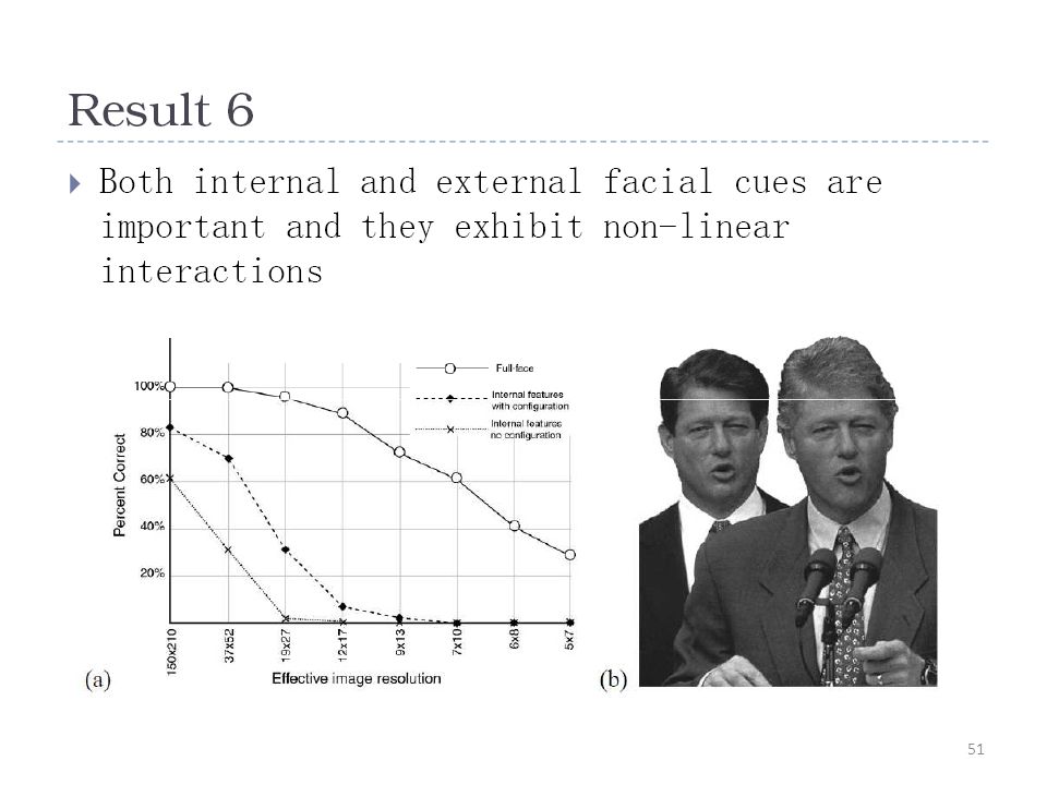
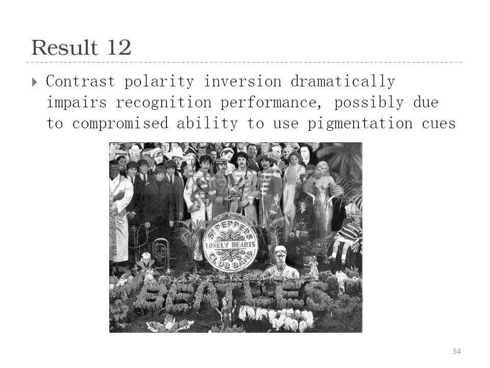
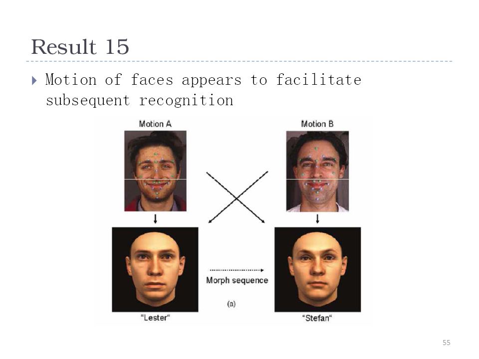
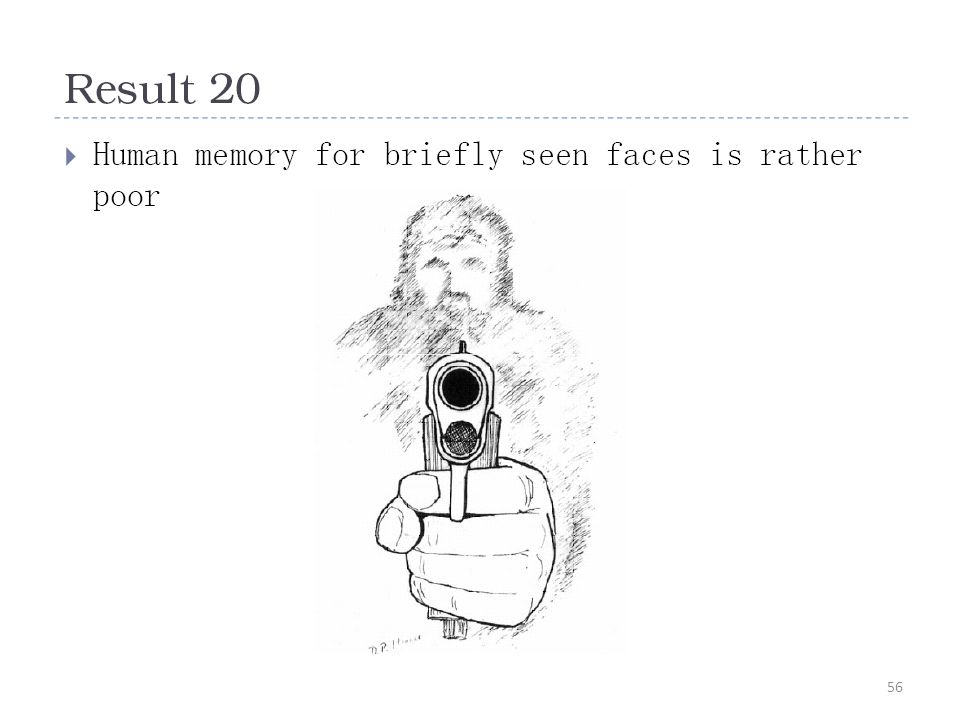
47. Face recognition by humans
Face recognition by humans: 20 results (2005)
Slides by Jianchao Yang

57. Things to remember
PCA is a generally useful dimensionality reduction technique
But not ideal for discrimination
FLD better for discrimination, though only ideal under Gaussian data assumptions
Computer face recognition works very well under controlled environments – still room for improvement in general conditions

58. Next class
Video processing

59. Questions?
See you Tuesday!
Slide credit: Devi Parikh