1. NumPy (and SciPy) Travis E. Oliphant Enthought, Inc.
Enthought, Inc.

2. What is NumPy? Python is a fabulous language Easy to extend
Great syntax which encourages easy to write and maintain code
Incredibly large standard-library and third-party tools
No built-in multi-dimensional array (but it supports the needed syntax for extracting elements from one)‏
NumPy provides a fast built-in object (ndarray) which is a multi-dimensional array of a homogeneous data-type.

3. NumPy Website -- http://numpy.scipy.org/
Offers Matlab-ish capabilities within Python
NumPy replaces Numeric and Numarray
Initially developed by Travis Oliphant (building on the work of dozens of others)
Over 30 svn “committers” to the project
NumPy 1.0 released October, 2006
~20K downloads/month from Sourceforge.
This does not count:
Linux distributions that include NumPy
Enthought distributions that include NumPy
Mac OS X distributions that include NumPy
Sage distributes that include NumPy

4. Overview of NumPy N-dimensional array of rectangular data
N-D ARRAY (NDARRAY)
UNIVERSAL FUNCTIONS (UFUNC)
N-dimensional array of rectangular data
Element of the array can be C-structure or simple data-type.
Fast algorithms on machine data-types (int, float, etc.)
functions that operate element-by-element and return result
fast-loops registered for each fundamental data-type
sin(x) = [sin(xi) i=0..N]
x+y = [xi + yi i=0..N]

5. NumPy Array
A NumPy array is an N-dimensional homogeneous collection of “items” of the same “kind”. The kind can be any arbitrary structure and is specified using the data-type.

6. NumPy Array
A NumPy array is a homogeneous collection of “items” of the same “data-type” (dtype)‏
>>> import numpy as N
>>> a = N.array([[1,2,3],[4,5,6]],float)‏
>>> print a
[[ ]
[ ]]
>>> print a.shape, ”\n”, a.itemsize
(2, 3)‏ 8
>>> print a.dtype, a.dtype.type
'<f8' <type 'float64scalar'>
>>> type(a[0,0])‏
<type 'float64scalar'>
>>> type(a[0,0]) is type(a[1,2])
True

7. Introducing NumPy Arrays
SIMPLE ARRAY CREATION
ARRAY SHAPE
>>> a = array([0,1,2,3])
>>> a
array([0, 1, 2, 3])
# shape returns a tuple
# listing the length of the
# array along each dimension.
>>> a.shape
(4,)
>>> shape(a)
# size reports the entire
# number of elements in an # array.
>>> a.size 4
>>> size(a)
CHECKING THE TYPE
>>> type(a)
<type 'array'>
NUMERIC ‘TYPE’ OF ELEMENTS
ARRAY SIZE
>>> a.dtype
dtype(‘int32’)
BYTES PER ELEMENT
>>> a.itemsize # per element 4

8. Introducing NumPy Arrays
BYTES OF MEMORY USED
CONVERSION TO LIST
# returns the number of bytes # used by the data portion of # the array.
>>> a.nbytes 12
# convert a numpy array to a
# python list.
>>> a.tolist()
[0, 1, 2, 3]
# For 1D arrays, list also
# works equivalently, but
# is slower.
>>> list(a)
NUMBER OF DIMENSIONS
>>> a.ndim 1
ARRAY COPY
# create a copy of the array
>>> b = a.copy()
>>> b
array([0, 1, 2, 3])

9. Setting Array Elements
ARRAY INDEXING
BEWARE OF TYPE COERSION
>>> a[0]
>>> a[0] = 10
>>> a
[10, 1, 2, 3]
>>> a.dtype
dtype('int32')
# assigning a float to into # an int32 array will
# truncate decimal part.
>>> a[0] = 10.6
>>> a
[10, 1, 2, 3]
# fill has the same behavior
>>> a.fill(-4.8)
[-4, -4, -4, -4]
FILL
# set all values in an array.
>>> a.fill(0)
>>> a
[0, 0, 0, 0]
# This also works, but may
# be slower.
>>> a[:] = 1
[1, 1, 1, 1]

10. Multi-Dimensional Arrays
NUMBER OF DIMENSIONS
>>> a = array([[ 0, 1, 2, 3],
[10,11,12,13]])
>>> a
array([[ 0, 1, 2, 3],
>>> a.ndims 2
GET/SET ELEMENTS
>>> a[1,3] 13
>>> a[1,3] = -1
>>> a
array([[ 0, 1, 2, 3],
[10,11,12,-1]])
column
(ROWS,COLUMNS)
row
>>> a.shape
(2, 4)
>>> shape(a)
ELEMENT COUNT
ADDRESS FIRST ROW USING SINGLE INDEX
>>> a.size 8
>>> size(a)
>>> a[1]
array([10, 11, 12, -1])

11. Array Slicing SLICING WORKS MUCH LIKE STANDARD PYTHON SLICING
[54, 55]])
>>> a[:,2]
array([2,12,22,32,42,52])
STRIDES ARE ALSO POSSIBLE
>>> a[2::2,::2]
array([[20, 22, 24],
[40, 42, 44]])

12. Memory Model
>>> print a.strides
(24, 8)‏
>>> print a.flags.fortran, a.flags.contiguous
False True
>>> print a.T.strides
(8, 24)‏
>>> print a.T.flags.fortran, a.T.flags.contiguous
True False
Every dimension of an ndarray is accessed by stepping (striding) a fixed number of bytes through memory.
If memory is contiguous, then the strides are “pre-computed” indexing-formulas for either Fortran-order (first-dimension varies the fastest), or C-order (last-dimension varies the fastest) arrays.

13. Array slicing (Views)‏
Memory model allows “simple indexing” (integers and slices) into the array to be a view of the same data.
Other uses of view
>>> b = a[:,::2]
>>> b[0,1] = 100
>>> print a
[[ ]]
[ ]]
>>> c = a[:,::2].copy()‏
>>> c[1,0] = 500
>>> b = a.view('i8')‏
>>> [hex(val.item()) for val in b.flat]
['0x3FF L',
'0x L',
'0x L',
'0x L',
'0x L',
'0x L']

14. Slices Are References >>> a = array((0,1,2,3,4))
Slices are references to memory in original array. Changing values in a slice also changes the original array.
>>> a = array((0,1,2,3,4))
# create a slice containing only the
# last element of a
>>> b = a[2:4]
>>> b[0] = 10
# changing b changed a!
>>> a
array([ 1, 2, 10, 3, 4])
Good
1. More efficient because it doesn’t force array copies for every operation.
2. It is often nice to rename the view of an array for manipulation. (A view of the odd and even arrays)
Bad
1. Can cause unexpected side-effects that are hard to track down.
2. When you would rather have a copy, it requires some ugliness.

15. Fancy Indexing a y INDEXING BY POSITION INDEXING WITH BOOLEANS
>>> a = arange(0,80,10)
# fancy indexing
>>> y = a[[1, 2, -3]]
>>> print y
[ ]
# using take
>>> y = take(a,[1,2,-3])
>>> mask = array([0,1,1,0,0,1,0,0],
dtype=bool)
# fancy indexing
>>> y = a[mask]
>>> print y
[10,20,50]
# using compress
>>> y = compress(mask, a) a y

16. Fancy Indexing in 2D >>> a[(0,1,2,3,4),(1,2,3,4,5)]
array([ 1, 12, 23, 34, 45])
>>> a[3:,[0, 2, 5]]
array([[30, 32, 35],
[40, 42, 45]])
[50, 52, 55]])
>>> mask = array([1,0,1,0,0,1],
dtype=bool)
>>> a[mask,2]
array([2,22,52])
Unlike slicing, fancy indexing creates copies instead of views into original arrays.

17. Data-types There are two related concepts of “type”
The data-type object (dtype)‏
The Python “type” of the object created from a single array item (hierarchy of scalar types)‏
The dtype object provides the details of how to interpret the memory for an item. It's an instance of a single dtype class.
The “type” of the extracted elements are true Python classes that exist in a hierarchy of Python classes
Every dtype object has a type attribute which provides the Python object returned when an element is selected from the array

18. NumPy dtypes Basic Type Available NumPy types Comments Boolean bool
Elements are 1 byte in size
Integer
int8, int16, int32, int64, int128, int
int defaults to the size of int in C for the platform
Unsigned Integer
uint8, uint16, uint32, uint64, uint128, uint
uint defaults to the size of unsigned int in C for the platform
Float
float32, float64, float, longfloat,
Float is always a double precision floating point value (64 bits). longfloat represents large precision floats. Its size is platform dependent.
Complex
complex64, complex128, complex
The real and complex elements of a complex64 are each represented by a single precision (32 bit) value for a total size of 64 bits.
Strings
str, unicode
Unicode is always UTF32 (UCS4)
Object
object
Represent items in array as Python objects.
Records
void
Used for arbitrary data structures in record arrays.

19. Built-in “scalar” types

20. Data-type object (dtype)‏
There are 21 “built-in” (static) data-type objects
New (dynamic) data-type objects are created to handle
Alteration of the byteorder
Change in the element size (for string, unicode, and void built-ins)‏
Addition of fields
Change of the type object (C-structure arrays)
Creation of data-types is quite flexible.
New user-defined “built-in” data-types can also be added (but must be done in C and involves filling a function-pointer table)‏

21. Data-type fields An item can include fields of different data-types.
A field is described by a data-type object and a byte offset --- this definition allows nested records.
The array construction command interprets tuple elements as field entries.
>>> dt = N.dtype(“i4,f8,a5”)‏
>>> print dt.fields
{'f1': (dtype('<i4'), 0), 'f2': (dtype('<f8'), 4), 'f3': (dtype('|S5'), 12)}
>>> a = N.array([(1,2.0,”Hello”), (2,3.0,”World”)], dtype=dt)‏
>>> print a['f3']
[Hello World]

22. Array Calculation Methods
SUM FUNCTION
SUM ARRAY METHOD
>>> a = array([[1,2,3],
[4,5,6]], float)
# Sum defaults to summing all
# *all* array values.
>>> sum(a)
21.
# supply the keyword axis to
# sum along the 0th axis.
>>> sum(a, axis=0)
array([5., 7., 9.])
# sum along the last axis.
>>> sum(a, axis=-1)
array([6., 15.])
# The a.sum() defaults to
# summing *all* array values
>>> a.sum()
21.
# Supply an axis argument to
# sum along a specific axis.
>>> a.sum(axis=0)
array([5., 7., 9.])
PRODUCT
# product along columns.
>>> a.prod(axis=0)
array([ 4., 10., 18.])
# functional form.
>>> prod(a, axis=0)

23. Min/Max
MIN
MAX
>>> a = array([2.,3.,0.,1.]) >>> a.min(axis=0) 0.
# use Numpy’s amin() instead
# of Python’s builtin min()
# for speed operations on
# multi-dimensional arrays.
>>> amin(a, axis=0)
>>> a = array([2.,1.,0.,3.]) >>> a.max(axis=0) 3.
# functional form
>>> amax(a, axis=0)
ARGMIN
ARGMAX
# Find index of minimum value.
>>> a.argmin(axis=0) 2
# functional form
>>> argmin(a, axis=0)
# Find index of maximum value.
>>> a.argmax(axis=0) 1
# functional form
>>> argmax(a, axis=0)

24. Statistics Array Methods
MEAN
STANDARD DEV./VARIANCE
>>> a = array([[1,2,3],
[4,5,6]], float)
# mean value of each column
>>> a.mean(axis=0)
array([ 2.5, 3.5, 4.5])
>>> mean(a, axis=0)
>>> average(a, axis=0)
# average can also calculate
# a weighted average
>>> average(a, weights=[1,2], axis=0)
array([ 3., 4., 5.])
# Standard Deviation
>>> a.std(axis=0)
array([ 1.5, 1.5, 1.5])
# Variance
>>> a.var(axis=0)
array([2.25, 2.25, 2.25])
>>> var(a, axis=0)

25. Other Array Methods CLIP ROUND POINT TO POINT
# Limit values to a range
>>> a = array([[1,2,3],
[4,5,6]], float)
# Set values < 3 equal to 3.
# Set values > 5 equal to 5.
>>> a.clip(3,5)
>>> a
array([[ 3., 3., 3.],
[ 4., 5., 5.]])
# Round values in an array.
# Numpy rounds to even, so
# 1.5 and 2.5 both round to 2.
>>> a = array([1.35, 2.5, 1.5])
>>> a.round()
array([ 1., 2., 2.])
# Round to first decimal place.
>>> a.round(decimals=1)
array([ 1.4, 2.5, 1.5])
POINT TO POINT
# Calculate max – min for
# array along columns
>>> a.ptp(axis=0)
array([ 3.0, 3.0, 3.0])
# max – min for entire array.
>>> a.ptp(axis=None)
5.0

26. Summary of (most) array attributes/methods
BASIC ATTRIBUTES
a.dtype – Numerical type of array elements. float32, uint8, etc.
a.shape – Shape of the array. (m,n,o,...)
a.size – Number of elements in entire array.
a.itemsize – Number of bytes used by a single element in the array.
a.nbytes – Number of bytes used by entire array (data only).
a.ndim – Number of dimensions in the array.
SHAPE OPERATIONS
a.flat – An iterator to step through array as if it is 1D.
a.flatten() – Returns a 1D copy of a multi-dimensional array.
a.ravel() – Same as flatten(), but returns a ‘view’ if possible.
a.resize(new_size) – Change the size/shape of an array in-place.
a.swapaxes(axis1, axis2) – Swap the order of two axes in an array. a.transpose(*axes) – Swap the order of any number of array axes. a.T – Shorthand for a.transpose()
a.squeeze() – Remove any length=1 dimensions from an array.
These are definitely summaries – I have not included all the arguments for functions in many cases.

27. Summary of (most) array attributes/methods
FILL AND COPY
a.copy() – Return a copy of the array.
a.fill(value) – Fill array with a scalar value.
CONVERSION / COERSION
a.tolist() – Convert array into nested lists of values.
a.tostring() – raw copy of array memory into a python string.
a.astype(dtype) – Return array coerced to given dtype.
a.byteswap(False) – Convert byte order (big <-> little endian).
COMPLEX NUMBERS
a.real – Return the real part of the array.
a.imag – Return the imaginary part of the array.
a.conjugate() – Return the complex conjugate of the array.
a.conj()– Return the complex conjugate of an array.(same as conjugate)

28. Summary of (most) array attributes/methods
SAVING
a.dump(file) – Store a binary array data out to the given file.
a.dumps() – returns the binary pickle of the array as a string.
a.tofile(fid, sep="", format="%s") Formatted ascii output to file.
SEARCH / SORT
a.nonzero() – Return indices for all non-zero elements in a.
a.sort(axis=-1) – Inplace sort of array elements along axis.
a.argsort(axis=-1) – Return indices for element sort order along axis. a.searchsorted(b) – Return index where elements from b would go in a.
ELEMENT MATH OPERATIONS
a.clip(low, high) – Limit values in array to the specified range.
a.round(decimals=0) – Round to the specified number of digits.
a.cumsum(axis=None) – Cumulative sum of elements along axis.
a.cumprod(axis=None) – Cumulative product of elements along axis.

29. Summary of (most) array attributes/methods
REDUCTION METHODS
All the following methods “reduce” the size of the array by 1 dimension by carrying out an operation along the specified axis. If axis is None, the operation is carried out across the entire array.
a.sum(axis=None) – Sum up values along axis.
a.prod(axis=None) – Find the product of all values along axis.
a.min(axis=None)– Find the minimum value along axis.
a.max(axis=None) – Find the maximum value along axis.
a.argmin(axis=None) – Find the index of the minimum value along axis.
a.argmax(axis=None) – Find the index of the maximum value along axis.
a.ptp(axis=None) – Calculate a.max(axis) – a.min(axis)
a.mean(axis=None) – Find the mean (average) value along axis.
a.std(axis=None) – Find the standard deviation along axis.
a.var(axis=None) – Find the variance along axis.
a.any(axis=None) – True if any value along axis is non-zero. (or)
a.all(axis=None) – True if all values along axis are non-zero. (and)

30. Array Operations SIMPLE ARRAY MATH MATH FUNCTIONS
>>> a = array([1,2,3,4])
>>> b = array([2,3,4,5])
>>> a + b
array([3, 5, 7, 9])
# Create array from 0 to 10
>>> x = arange(11.)
# multiply entire array by
# scalar value
>>> a = (2*pi)/10.
>>> a
>>> a*x
array([ 0.,0.628,…,6.283])
# inplace operations
>>> x *= a
>>> x
# apply functions to array.
>>> y = sin(x)
Numpy defines the following constants:
pi =
e =

31. Universal Functions
ufuncs are objects that rapidly evaluate a function element-by-element over an array.
Core piece is a 1-d loop written in C that performs the operation over the largest dimension of the array
For 1-d arrays it is equivalent to but much faster than list comprehension
>>> type(N.exp)‏
<type 'numpy.ufunc'>
>>> x = array([1,2,3,4,5])‏
>>> print N.exp(x)‏
[ ]
>>> print [math.exp(val) for val in x]
[ , , ,
, ]

32. Mathematic Binary Operators
a + b  add(a,b)
a - b  subtract(a,b)
a % b  remainder(a,b)
a * b  multiply(a,b)
a / b  divide(a,b)
a ** b  power(a,b)
MULTIPLY BY A SCALAR
ADDITION USING AN OPERATOR FUNCTION
>>> a = array((1,2))
>>> a*3.
array([3., 6.])
>>> add(a,b)
array([4, 6])
ELEMENT BY ELEMENT ADDITION
IN PLACE OPERATION
# Overwrite contents of a.
# Saves array creation # overhead
>>> add(a,b,a) # a += b
array([4, 6])
>>> a
>>> a = array([1,2])
>>> b = array([3,4])
>>> a + b
array([4, 6])

33. Comparison and Logical Operators
equal (==)
greater_equal (>=)
logical_and
logical_not
not_equal (!=)
less (<)
logical_or
greater (>)
less_equal (<=)
logical_xor
2D EXAMPLE
>>> a = array(((1,2,3,4),(2,3,4,5)))
>>> b = array(((1,2,5,4),(1,3,4,5)))
>>> a == b
array([[True, True, False, True],
[False, True, True, True]])
# functional equivalent
>>> equal(a,b)

34. Bitwise Operators Bitwise operators only work on Integer arrays.
bitwise_and (&)
bitwise_or (|)
invert (~)
bitwise_xor
right_shift(a,shifts)
left_shift (a,shifts)
BITWISE EXAMPLES
>>> a = array((1,2,4,8))
>>> b = array((16,32,64,128))
>>> bitwise_or(a,b)
array([ 17, 34, 68, 136])
# bit inversion
>>> a = array((1,2,3,4), uint8)
>>> invert(a)
array([254, 253, 252, 251], dtype=uint8)
# left shift operation
>>> left_shift(a,3)
array([ 8, 16, 24, 32], dtype=uint8)
Bitwise operators only work on Integer arrays.
note: invert means bitwise_not (there is not a bitwise_not operator) -- probably should be though. invert is ambiguous. bitwise_not isn’t.
?? Why does left_shift convert the array from ‘b’ to ‘i’?

35. Trig and Other Functions
TRIGONOMETRIC
OTHERS
sin(x) sinh(x)
cos(x) cosh(x)
arccos(x) arccosh(x)
arctan(x) arctanh(x)
arcsin(x) arcsinh(x)
arctan2(x,y)
exp(x) log(x)
log10(x) sqrt(x)
absolute(x) conjugate(x)
negative(x) ceil(x)
floor(x) fabs(x) hypot(x,y) fmod(x,y) maximum(x,y) minimum(x,y)
hypot(x,y)
difference between fabs, abs,absolute?
timing wise, fabs is about twice as slow on
Windows 2K as the other two. yikes!!
Element by element distance
calculation using

36. Broadcasting
When there are multiple inputs, then they all must be “broadcastable” to the same shape.
All arrays are promoted to the same number of dimensions (by pre-prending 1's to the shape)‏
All dimensions of length 1 are expanded as determined by other inputs with non-unit lengths in that dimension.
>>> x = [1,2,3,4];
>>> y = [[10],[20],[30]]
>>> print N.add(x,y)‏
[[ ]
[ ]
[ ]]
>>> x = array(x)‏
>>> y = array(y)‏
>>> print x+y
x has shape (4,) the ufunc sees it as having shape (1,4)‏
y has shape (3,1)‏
The ufunc result has shape (3,4)

37. Array Broadcasting
4x3
4x3
4x3 3
stretch
4x1 3
stretch
stretch

38. Broadcasting Rules
The trailing axes of both arrays must either be 1 or have the same size for broadcasting to occur. Otherwise, a “ValueError: frames are not aligned” exception is thrown.
mismatch!
4x3 4

39. Broadcasting in Action
>>> a = array((0,10,20,30))
>>> b = array((0,1,2))
>>> y = a[:, None] + b

40. Universal Function Methods
The mathematic, comparative, logical, and bitwise operators that
take two arguments (binary operators) have special methods that operate on arrays:
op.reduce(a,axis=0)
op.accumulate(a,axis=0)
op.outer(a,b)
op.reduceat(a,indices)

41. Vectorizing Functions
Example
# attempt
>>> sinc([1.3,1.5])
TypeError: can't multiply sequence to non-int
>>> x = r_[-5:5:100j]
>>> y = vsinc(x)
>>> plot(x, y)
# special.sinc already available
# This is just for show.
def sinc(x):
if x == 0.0:
return 1.0
else:
w = pi*x
return sin(w) / w
SOLUTION
>>> from numpy import vectorize
>>> vsinc = vectorize(sinc)
>>> vsinc([1.3,1.5])
array([ , ])

42. Interface with C/C++/Fortan
Python excels at interfacing with other languages
weave (C/C++)‏
f2py (Fortran)‏
pyrex
ctypes (C)‏
SWIG (C/C++)‏
Boost.Python (C++)‏
RPy / RSPython (R)‏

43. Matplotlib http://matplotlib.sourceforge.net
Requires NumPy extension. Provides powerful plotting commands.

44. Recommendations
Matplotlib for day-to-day data exploration. Matplotlib has a large community, tons of plot types, and is well integrated into ipython. It is the de-facto standard for ‘command line’ plotting from ipython.
Chaco for building interactive plotting applications Chaco is architected for building highly interactive and configurable plots in python. It is more useful as plotting toolkit than for making one-off plots.

45. Line Plots PLOT AGAINST INDICES MULTIPLE DATA SETS
>>> x = arange(50)*2*pi/50.
>>> y = sin(x)
>>> plot(y)
>>> xlabel(‘index’)
>>> plot(x,y,x2,y2)
>>> xlabel(‘radians’)

46. Line Plots LINE FORMATTING MULTIPLE PLOT GROUPS
# red, dot-dash, triangles
>>> plot(x,sin(x),'r-^')
>>> plot(x,y1,'b-o', x,y2), r-^')
>>> axis([0,7,-2,2])

47. Scatter Plots SIMPLE SCATTER PLOT COLORMAPPED SCATTER
>>> x = arange(50)*2*pi/50.
>>> y = sin(x)
>>> scatter(x,y)
# marker size/color set with data
>>> x = rand(200)
>>> y = rand(200)
>>> size = rand(200)*30
>>> color = rand(200)
>>> scatter(x, y, size, color)
>>> colorbar()

48. Bar Plots BAR PLOT HORIZONTAL BAR PLOT >>> bar(x,sin(x),
width=x[1]-x[0])
>>> hbar(x,sin(x),
height=x[1]-x[0],
orientation=‘horizontal’)

49. Bar Plots
DEMO/MATPLOTLIB_PLOTTING/BARCHART_DEMO.PY

50. HISTOGRAMS HISTOGRAM HISTOGRAM 2 # plot histogram # default to 10 bins
>>> hist(randn(1000))
# change the number of bins
>>> hist(randn(1000), 30)

51. Multiple Plots using Subplot
DEMO/MATPLOTLIB_PLOTTING/EXAMPLES/SUBPLOT_DEMO.PY
def f(t):
s1 = cos(2*pi*t)
e1 = exp(-t)
return multiply(s1,e1)
t1 = arange(0.0, 5.0, 0.1)
t2 = arange(0.0, 5.0, 0.02)
t3 = arange(0.0, 2.0, 0.01)
subplot(211)
l = plot(t1, f(t1), 'bo', t2, f(t2), 'k--')
setp(l, 'markerfacecolor', 'g')
grid(True)
title('A tale of 2 subplots')
ylabel('Damped oscillation')
subplot(212)
plot(t3, cos(2*pi*t3), 'r.')
xlabel('time (s)')
ylabel('Undamped')
show()

52. Image Display # Create 2d array where values
# are radial distance from
# the center of array.
>>> from numpy import mgrid
>>> from scipy import special
>>> x,y = mgrid[-25:25:100j,
:25:100j]
>>> r = sqrt(x**2+y**2)
# Calculate bessel function of
# each point in array and scale
>>> s = special.j0(r)*25
# Display surface plot.
>>> imshow(s, extent=[-25,25,-25,25])
>>> colorbar()

53. Surface plots with mlab
# Create 2d array where values
# are radial distance from
# the center of array.
>>> from numpy import mgrid
>>> from scipy import special
>>> x,y = mgrid[-25:25:100j,
:25:100j]
>>> r = sqrt(x**2+y**2)
# Calculate bessel function of
# each point in array and scale
>>> s = special.j0(r)*25
# Display surface plot.
>>> from enthought.mayavi \ import mlab
>>> mlab.surf(x,y,s)
>>> mlab.scalarbar()
>>> mlab.axes()

54. SciPy Overview Available at www.scipy.org
Open Source BSD Style License
Over 30 svn “committers” to the project
CURRENT PACKAGES
Special Functions (scipy.special)
Signal Processing (scipy.signal)
Image Processing (scipy.ndimage)
Fourier Transforms (scipy.fftpack)
Optimization (scipy.optimize)
Numerical Integration (scipy.integrate)
Linear Algebra (scipy.linalg)
Input/Output (scipy.io)
Statistics (scipy.stats)
Fast Execution (scipy.weave)
Clustering Algorithms (scipy.cluster)
Sparse Matrices (scipy.sparse)
Interpolation (scipy.interpolate)
More (e.g. scipy.odr, scipy.maxentropy)

55. 1D Spline Interpolation
# demo/interpolate/spline.py
from scipy.interpolate import interp1d
from pylab import plot, axis, legend
from numpy import linspace
# sample values
x = linspace(0,2*pi,6)
y = sin(x)
# Create a spline class for interpolation.
# kind=5 sets to 5th degree spline.
# kind=0 -> zeroth order hold.
# kind=1 or ‘linear’ -> linear interpolation
# kind=2 or
spline_fit = interp1d(x,y,kind=5)
xx = linspace(0,2*pi, 50)
yy = spline_fit(xx)
# display the results.
plot(xx, sin(xx), 'r-', x,y,'ro',xx,yy, 'b--',linewidth=2)
axis('tight')
legend(['actual sin', 'original samples', 'interpolated curve'])

56. FFT scipy.fft --- FFT and related functions
>>> n = fftfreq(128)*128
>>> f = fftfreq(128)
>>> ome = 2*pi*f
>>> x = (0.9)**abs(n)
>>> X = fft(x)
>>> z = exp(1j*ome)
>>> Xexact = (0.9**2 - 1)/0.9*z / \
(z-0.9) / (z-1/0.9)
>>> f = fftshift(f)
>>> plot(f, fftshift(X.real),'r-',
f, fftshift(Xexact.real),'bo')
>>> title('Fourier Transform Example')
>>> xlabel('Frequency (cycles/s)')
>>> axis(-0.6,0.6, 0, 20)

57. FFT EXAMPLE --- Short-Time Windowed Fourier Transform
rate, data = read('scale.wav')
dT, T_window = 1.0/rate, 50e-3
N_window = int(T_window * rate)
N_data = len(data)
window = get_window('hamming', N_window)
result, start = [], 0
# compute short-time FFT for each block
while (start < N_data – N_window):
end = start + N_window
val = fftshift(fft(window*data[start:end]))
result.append(val)
start = end
lastval = fft(window*data[-N_window:])
result.append(fftshift(lastval))
result = array(result,result[0].dtype)

58. Signal Processing What’s Available?
scipy.signal --- Signal and Image Processing
What’s Available?
Filtering
General 2-D Convolution (more boundary conditions)
N-D convolution
B-spline filtering
N-D Order filter, N-D median filter, faster 2d version,
IIR and FIR filtering and filter design
LTI systems
System simulation
Impulse and step responses
Partial fraction expansion

59. Image Processing LENA IMAGE MEDIAN FILTERED IMAGE
# The famous lena image is packaged with scipy
>>> from scipy import lena, signal
>>> lena = lena().astype(float32)
>>> imshow(lena, cmap=cm.gray)
# Blurring using a median filter
>>> fl = signal.medfilt2d(lena, [15,15])
>>> imshow(fl, cmap=cm.gray)
LENA IMAGE
MEDIAN FILTERED IMAGE

60. Image Processing NOISY IMAGE FILTERED IMAGE
# Noise removal using wiener filter
>>> from scipy.stats import norm
>>> ln = lena + norm(0,32).rvs(lena.shape)
>>> imshow(ln)
>>> cleaned = signal.wiener(ln)
>>> imshow(cleaned)
NOISY IMAGE
FILTERED IMAGE

61. Image Processing NOISY IMAGE FILTERED IMAGE
# Edge detection using Sobel filter
>>> from scipy.ndimage.filters import sobel
>>> imshow(lena)
>>> edges = sobel(lena)
>>> imshow(edges)
NOISY IMAGE
FILTERED IMAGE

62. LTI Systems >>> b,a = [1],[1,6,25]
>>> ltisys = signal.lti(b,a)
>>> t,h = ltisys.impulse()
>>> ts,s = ltisys.step()
>>> plot(t,h,ts,s)
>>> legend(['Impulse response','Step response'])

63. Optimization Unconstrained Optimization Constrained Optimization
scipy.optimize --- unconstrained minimization and root finding
Unconstrained Optimization
fmin (Nelder-Mead simplex), fmin_powell (Powell’s method), fmin_bfgs (BFGS quasi-Newton method), fmin_ncg (Newton conjugate gradient), leastsq (Levenberg-Marquardt), anneal (simulated annealing global minimizer), brute (brute force global minimizer), brent (excellent 1-D minimizer), golden, bracket
Constrained Optimization
fmin_l_bfgs_b, fmin_tnc (truncated newton code), fmin_cobyla (constrained optimization by linear approximation), fminbound (interval constrained 1-d minimizer)
Root finding
fsolve (using MINPACK), brentq, brenth, ridder, newton, bisect, fixed_point (fixed point equation solver)

64. Optimization EXAMPLE: MINIMIZE BESSEL FUNCTION
# minimize 1st order bessel
# function between 4 and 7
>>> from scipy.special import j1
>>> from scipy.optimize import \ fminbound
>>> x = r_[2:7.1:.1]
>>> j1x = j1(x)
>>> plot(x,j1x,’-’)
>>> hold(True)
>>> x_min = fminbound(j1,4,7)
>>> j1_min = j1(x_min)
>>> plot([x_min],[j1_min],’ro’)

65. Optimization EXAMPLE: SOLVING NONLINEAR EQUATIONS
Solve the non-linear equations
>>> def nonlin(x,a,b,c):
>>> x0,x1,x2 = x
>>> return [3*x0-cos(x1*x2)+ a,
>>> x0*x0-81*(x1+0.1)** sin(x2)+b,
>>> exp(-x0*x1)+20*x2+c]
>>> a,b,c = -0.5,1.06,(10*pi-3.0)/3
>>> root = optimize.fsolve(nonlin, [0.1,0.1,-0.1],args=(a,b,c))
>>> print root
[ ]
>>> print nonlin(root,a,b,c)
[0.0, e-12, e-14]
starting location for search

66. Optimization EXAMPLE: MINIMIZING ROSENBROCK FUNCTION
WITHOUT DERIVATIVE
USING DERIVATIVE
>>> rosen = optimize.rosen
>>> import time
>>> x0 = [1.3,0.7,0.8,1.9,1.2]
>>> start = time.time()
>>> xopt = optimize.fmin(rosen,
x0, avegtol=1e-7)
>>> stop = time.time()
>>> print_stats(start, stop, xopt)
Optimization terminated successfully.
Current function value:
Iterations: 316
Function evaluations: 533
Found in seconds
Solution: [ ]
Function value: e-15
Avg. Error: e-08
>>> rosen_der = optimize.rosen_der
>>> x0 = [1.3,0.7,0.8,1.9,1.2]
>>> start = time.time()
>>> xopt = optimize.fmin_bfgs(rosen,
x0, fprime=rosen_der, avegtol=1e-7)
>>> stop = time.time()
>>> print_stats(start, stop, xopt)
Optimization terminated successfully.
Current function value:
Iterations: 111
Function evaluations: 266
Gradient evaluations: 112
Found in seconds
Solution: [ ]
Function value: e-18
Avg. Error: e-10

67. Optimization EXAMPLE: Non-linear least-squares data fitting
# fit data-points to a curve
# demo/data_fitting/datafit.py
>>> from numpy.random import randn
>>> from numpy import exp, sin, pi
>>> from numpy import linspace
>>> from scipy.optimize import leastsq
>>> def func(x,A,a,f,phi):
return A*exp(-a*sin(f*x+pi/4))
>>> def errfunc(params, x, data):
return func(x, *params) - data
>>> ptrue = [3,2,1,pi/4]
>>> x = linspace(0,2*pi,25)
>>> true = func(x, *ptrue)
>>> noisy = true + 0.3*randn(len(x))
>>> p0 = [1,1,1,1]
>>> pmin, ier = leastsq(errfunc, p0,
args=(x, noisy))
>>> pmin
array([3.1705, , , ])

68. Statistics scipy.stats --- CONTINUOUS DISTRIBUTIONS
over 80 continuous distributions!
METHODS
pdf
cdf
rvs
ppf
stats

69. Statistics scipy.stats --- Discrete Distributions
10 standard discrete distributions (plus any arbitrary finite RV)
METHODS
pdf
cdf
rvs
ppf
stats

70. Using stats objects DISTRIBUTIONS # Sample normal dist. 100 times.
>>> samp = stats.norm.rvs(size=100)
>>> x = r_[-5:5:100j]
# Calculate probability dist.
>>> pdf = stats.norm.pdf(x)
# Calculate cummulative Dist.
>>> cdf = stats.norm.cdf(x)
# Calculate Percent Point Function
>>> ppf = stats.norm.ppf(x)

71. Statistics scipy.stats --- Basic Statistical Calculations on Data
numpy.mean, numpy.std, numpy.var, numpy.cov
stats.skew, stats.kurtosis, stats.moment
scipy.stats.bayes_mvs --- Bayesian mean, variance, and std.
# Create “frozen” Gamma distribution with a=2.5
>>> grv = stats.gamma(2.5)
>>> grv.stats() # Theoretical mean and variance
(array(2.5), array(2.5))
# Estimate mean, variance, and std with 95% confidence
>>> vals = grv.rvs(size=100)
>>> stats.bayes_mvs(vals, alpha=0.95)
(( , ( , )),
( , ( , )),
( , ( , )))
# (expected value and confidence interval for each of
# mean, variance, and standard-deviation)

72. Using stats objects CREATING NEW DISCRETE DISTRIBUTIONS
# Create a loaded dice.
>>> from scipy.stats import rv_discrete
>>> xk = [1,2,3,4,5,6]
>>> pk = [0.3,0.35,0.25,0.05,
0.025,0.025]
>>> new = rv_discrete(name='loaded',
values=(xk,pk))
# Calculate histogram
>>> samples = new.rvs(size=1000)
>>> bins=linspace(0.5,5.5,6)
>>> subplot(211)
>>> hist(samples,bins=bins,normed=True)
# Calculate pmf
>>> x = range(0,8)
>>> subplot(212)
>>> stem(x,new.pmf(x))

73. Statistics
Continuous PDF Estimation using Gaussian Kernel Density Estimation
# Sample normal dist. 100 times.
>>> rv1 = stats.norm()
>>> rv2 = stats.norm(2.0,0.8)
>>> samp = r_[rv1.rvs(size=100),
rv2.rvs(size=100)]
# Kernel estimate (smoothed histogram)
>>> apdf = stats.kde.gaussian_kde(samp)
>>> x = linspace(-3,6,200)
>>> plot(x, apdf(x),’r’)
# Histogram
>>> hist(x, bins=25, normed=True)

74. Linear Algebra Uses ATLAS if available --- very fast
scipy.linalg --- FAST LINEAR ALGEBRA
Uses ATLAS if available --- very fast
Low-level access to BLAS and LAPACK routines in modules linalg.fblas, and linalg.flapack (FORTRAN order)
High level matrix routines
Linear Algebra Basics: inv, solve, det, norm, lstsq, pinv
Decompositions: eig, lu, svd, orth, cholesky, qr, schur
Matrix Functions: expm, logm, sqrtm, cosm, coshm, funm (general matrix functions)

75. Linear Algebra LU FACTORIZATION EIGEN VALUES AND VECTORS
>>> from scipy import linalg
>>> a = array([[1,3,5],
[2,5,1],
[2,3,6]])
# time consuming factorization
>>> lu, piv = linalg.lu_factor(a)
# fast solve for 1 or more
# right hand sides.
>>> b = array([10,8,3])
>>> linalg.lu_solve((lu, piv), b)
array([ , , ])
>>> from scipy import linalg
>>> a = array([[1,3,5],
[2,5,1],
[2,3,6]])
# compute eigen values/vectors
>>> vals, vecs = linalg.eig(a)
# print eigen values
>>> vals
array([ j,
j, j])
# eigen vectors are in columns
# print first eigen vector
>>> vecs[:,0]
array([ , , ])
# norm of vector should be 1.0
>>> linalg.norm(vecs[:,0])
1.0

76. Matrix Objects STRING CONSTRUCTION DIAGONAL TRANSPOSE ATTRIBUTE SOLVE
>>> from numpy import mat
>>> a = mat('[1,3,5;2,5,1;2,3,6]')
>>> a
matrix([[1, 3, 5],
[2, 5, 1],
[2, 3, 6]])
>>> a.diagonal()
matrix([[1, 5, 6]])
>>> a.diagonal(-1)
matrix([[3, 1]])
TRANSPOSE ATTRIBUTE
SOLVE
>>> a.T
matrix([[1, 2, 2],
[3, 5, 3],
[5, 1, 6]])
>>> b = mat('10;8;3')
>>> a.I*b
matrix([[ ],
[ ],
[ ]])
>>> from scipy import linalg
>>> linalg.solve(a,b)
INVERTED ATTRIBUTE
>>> a.I
matrix([[ , , ],
[ , , ],
[ , , ] ])
# note: reformatted to fit slide

77. Integration Ordinary Differential Equations (ODE)
scipy.integrate --- General purpose Integration
Ordinary Differential Equations (ODE)
integrate.odeint, integrate.ode
Samples of a 1-d function
integrate.trapz (trapezoidal Method), integrate.simps (Simpson Method), integrate.romb (Romberg Method)
Arbitrary callable function
integrate.quad (general purpose), integrate.dblquad (double integration), integrate.tplquad (triple integration), integrate.fixed_quad (fixed order Gaussian integration), integrate.quadrature (Gaussian quadrature to tolerance), integrate.romberg (Romberg)

78. Integration scipy.integrate --- Example # Compare sin to integral(cos)
>>> def func(x):
return integrate.quad(cos,0,x)[0]
>>> vecfunc = vectorize(func)
>>> x = r_[0:2*pi:100j]
>>> x2 = x[::5]
>>> y = sin(x)
>>> y2 = vecfunc(x2)
>>> plot(x,y,x2,y2,'rx')
>>> legend([‘Exact‘,
‘Integral Result’])
# compute short-time FFT
# compute short-time FFT # compute short-time FFT

79. Special Functions Includes over 200 functions: scipy.special
Airy, Elliptic, Bessel, Gamma, HyperGeometric, Struve, Error, Orthogonal Polynomials, Parabolic Cylinder, Mathieu, Spheroidal Wave, Kelvin
FIRST ORDER BESSEL EXAMPLE
>>> from scipy import special
>>> x = r_[0:100:0.1]
>>> j0x = special.j0(x)
>>> plot(x,j0x)

80. Special Functions scipy.special AIRY FUNCTIONS EXAMPLE
>>> z = r_[-5:1.5:100j]
>>> vals = special.airy(z)
>>> plot(z,array(vals).T)
>>> legend(['Ai', 'Aip', ‘Bi‘,'Bip'])
>>> xlabel('z’)
>>> title('Airy Functions and Derivatives‘)

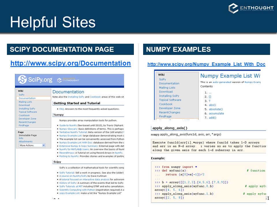
81. Helpful Sites SCIPY DOCUMENTATION PAGE NUMPY EXAMPLES

82. PyLab IPython SciPy Matplotlib NumPy Python
Sometimes the union of the 5 packages is called pylab: ipython -pylab.
Literally 1000's more modules/packages for Python
PMV
PIL
IPython
MayaVi
VTK
SciPy
Matplotlib
DejaVu
RPy
PMV
NumPy
ETS
ViPEr
Python
MolKit
Pygame

83. Extras: MayaVi
Prabu
Ramanchandran

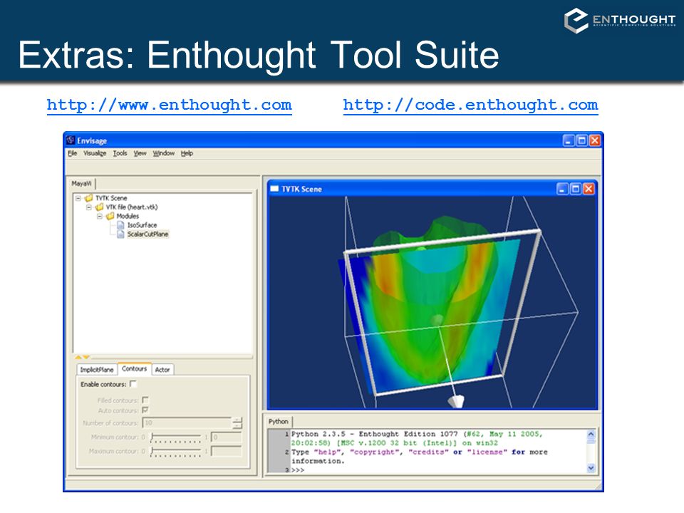
84. Extras: Enthought Tool Suite

85. You can get involved New algorithms in SciPy
Documentation improvements
Community interaction (mailing lists and bug tracker)
SciPy conference 2008 at Caltech in Pasadena, CA (August 19-24)