Download presentation
Presentation is loading. Please wait.

1
Psyc 235: Introduction to Statistics DON’T FORGET TO SIGN IN FOR CREDIT! http://www.psych.uiuc.edu/~jrfinley/p235/
2
(Not) Relationships among Variables Descriptive stats (e.g., mean, median, mode, standard deviation) describe a sample of data z-test &/or t-test for a single population parameter (e.g., mean) infer the true value of a single variable ex: mean # of random digits that people can memorize
 Relationships among Variables Descriptive stats (e.g., mean, median, mode, standard deviation) describe a sample of data z-test &/or t-test for a single population parameter (e.g., mean) infer the true value of a single variable ex: mean # of random digits that people can memorize")
3
Relationships among Variables But relationships among more than one variable are the crucial feature of almost all scientific research. Examples: How does the perception of a stimulus vary with the physical intensity of that stimulus? How does the attitude towards the President vary with the socio-economic properties of the survey respondent? How does the performance on a mental task vary with age?

4
Relationships among Variables More Examples: How does depression vary with number of traumatic experiences? How does undergraduate drinking vary with performance in quantitative courses? How does memory performance vary with attention span? etc... We’ve already learned a few ways to analyze relationships among 2 variables.

5
Relationships among Two Variables: Chi-Square Chi-Square test of independence (2-way contingency table) compare observed cell frequencies to the cell frequencies you’d expect if the two variables are independent. ex: X=geographical region: West coast, Midwest, East coast Y=favorite color: red, blue, green Note: both variables are categorical

6
Relationships among Two Variables: Chi-Square Observed frequencies: Expected frequencies:

7
Relationships among Two Variables: Chi-Square Observed frequencies: Expected frequencies: ≈17.97 if this exceeds critical value, reject H 0 that the 2 variables are independent (unrelated)
")
8
Relationships among Two Variables: z, t tests z-test &/or t-test for difference of population means compare values of one variable (Y) for 2 different levels/groups of another variable (X) ex: X=age: young people vs. old people Y=# random digits can memorize Q: Is the mean # digits the same for the 2 age groups?

9
Relationships among Two Variables: ANOVA ANOVA compare values of one variable (Y) for 3+ different levels/groups of another variable (X) ex: X=age: young people, middle-aged, old people Y=# random digits can memorize Q: Is the mean # digits the same for all 3 age groups?
 for 3+ different levels/groups of another variable (X) ex: X=age: young people, middle-aged, old people Y=# random digits can memorize Q: Is the mean # digits the same for all 3 age groups")
10
Relationships among Two Variables: z, t & ANOVA NOTE: for z/t tests for differences, and for ANOVA, there are a small number of possible values for one of the variables (X) z, t ANOVA
 z, t ANOVA")
11
Relationships among Two Variables: z, t & ANOVA NOTE: for z/t tests for differences, and for ANOVA, there are a small number of possible values for one of the variables (X) z, t ANOVA
 z, t ANOVA")
12
Relationships among Two Variables: many values of X? What about when there are many possible values of BOTH variables? Maybe they’re even continuous (rather than discrete)? Correlation, and Simple Linear Regression will be used to analyze relationship among two such variables (scatter plot)
. Correlation, and Simple Linear Regression will be used to analyze relationship among two such variables (scatter plot).")
13
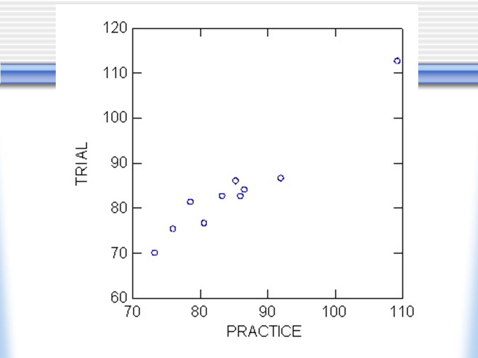
Correlation: Scatter Plots Does it look like there is a relationship?

14
Correlation measures the direction and strength of a linear relationship between two variables that is, it answers in a general way the question: “as the values of one variable change, how do the corresponding values of the other variable change?”

15
Linear Relationship linear relationship: y=a +bx (straight line) Linear Not (strictly) Linear
 Linear Not (strictly) Linear")
16
Correlation Coefficient: r sign: direction of relationship magnitude (number): strength of relationship -1 ≤ r ≤ 1 r=0 is no linear relationship r=-1 is “perfect” negative correlation r=1 is “perfect” positive correlation Notes: Symmetric Measure (You can exchange X and Y and get the same value) Measures linear relationship only
: strength of relationship -1 ≤ r ≤ 1 r=0 is no linear relationship r=-1 is perfect negative correlation r=1 is perfect positive correlation Notes: Symmetric Measure (You can exchange X and Y and get the same value) Measures linear relationship only")
17
Correlation Coefficient: r Formula: alt. formula (ALEKS): standardized values
: standardized values")
18
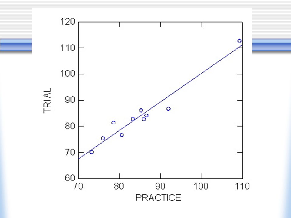
Correlation: Examples Population: undergraduates

19
Correlation: Examples Population: undergraduates

20
Correlation: Examples Population: undergraduates

21
Correlation: Examples Others?

22
Correlation: Interpretation Correlation ≠ Causation!

25
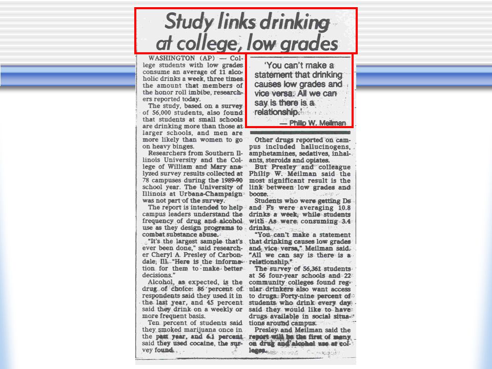
Correlation: Interpretation Correlation ≠ Causation! When 2 variables are correlated, the causality may be: X --> Y X <-- Y Z --> X&Y (“lurking” third variable) or a combination of the above Examples: ice cream & murder, violence & video games, SAT verbal & math, booze & GPA Inferring causation requires consideration of: how data gathered (e.g., experiment vs. observation), other relevant knowledge, logic...
 or a combination of the above Examples: ice cream & murder, violence & video games, SAT verbal & math, booze & GPA Inferring causation requires consideration of: how data gathered (e.g., experiment vs. observation), other relevant knowledge, logic....")
26
Simple Linear Regression PREDICTING one variable (Y) from another (X) No longer symmetric like Correlation One variable is used to “explain” another variable X Variable Independent Variable Explaining Variable Exogenous Variable Predictor Variable Y Variable Dependent Variable Response Variable Endogenous Variable Criterion Variable
 from another (X) No longer symmetric like Correlation One variable is used to explain another variable X Variable Independent Variable Explaining Variable Exogenous Variable Predictor Variable Y Variable Dependent Variable Response Variable Endogenous Variable Criterion Variable")
27
Simple Linear Regression idea: find a line (linear function) that best fits the scattered data points this will let us characterize the relationship between X & Y, and predict new values of Y for a given X value.
 that best fits the scattered data points this will let us characterize the relationship between X & Y, and predict new values of Y for a given X value.")
30
(0,a) b Intercept Slope bX+a X Reminder: (Simple) Linear Function Y=a+bX We are interested in this to model the relationship between an independent variable X and a dependent variable Y Y
 b Intercept Slope bX+a X Reminder: (Simple) Linear Function Y=a+bX We are interested in this to model the relationship between an independent variable X and a dependent variable Y Y")
31
1 X Y Simple Linear Regression all data points would fall right on the line

32
X Y A guess at the location of the regression line

33
X Y Another guess at the location of the regression line (same slope, different intercept)
")
34
X Y Initial guess at the location of the regression line

35
X Y Another guess at the location of the regression line (same intercept, different slope)
")
36
X Y Initial guess at the location of the regression line

37
X Y Another guess at the location of the regression line (different intercept and slope, same “center”)
")
38
X Y We will end up being reasonably confident that the true regression line is somewhere in the indicated region.

39
X Y Estimated Regression Line errors/residuals

40
X Y Estimated Regression Line

41
X Y Wrong Picture! Error Terms have to be drawn vertically

42
X Y Estimated Regression Line =“y hat”: predicted value of Y for X i

43
Estimating the Regression Line Idea: find the formula for the line that minimizes the squared errors error: distance between actual data point and predicted value Y=a+bX Y=b 0 +b 1 x b 1 =slope of regression line b 0 =Y intercept of regression line

44
ALEKS: Y=b 0 +b 1 X b 1 (slope) b 0 (Y intercept) using correlation coefficient
 b 0 (Y intercept) using correlation coefficient")
Similar presentations


 –new terms and concepts –assumptions –reading regression computer outputs Correlation.>")


