1. Dual Evolution for Geometric Reconstruction Huaiping Yang (FSP Project S09202) Johannes Kepler University of Linz 1 st FSP-Meeting in Graz, Nov. 23-25, 2005

3. Overview Introduction Outline of our method Evolution equation Synchronization of dual representations Refine the evolution result Experimental Results Conclusions

4. Introduction Geometric reconstruction from discrete point data sets has various applications: Two types of representations: Parametric curves/surfaces. Implicit curves/surfaces We use a combination of both representaions. Improved handling of both topology changes and shape constraints

5. Outline of our method We restrict our discussion to 2D cases: B-spline curves T-spline level sets Outline of our dual evolution: Initialization (pre-compute the evolution speed function) Evolution and synchronization (until some stopping criterion is satisfied) Refinement

6. Evolution equation We want to move the active curve (parametric or implicit) along its normal directions: - Points on the curve - Time variable - Unit normal vector - Evolution speed function -

7. Evolution speed function For image contour detection, we use a modified version of that proposed by Caselles et al. [Caselles1997]: For unorganized data points fitting, we use:

8. Parametric curve evolution B-spline curve representation: From evolution equation: we get, a discretized version of each evolution step can be formulated as a least squares problem:

9. Implicit curve evolution We use implicit T-spline curves [Sederberg2003], and is the T-spline function, where, are cubic B-spline basis functions associated with knot vectors,

10. Implicit curve evolution During the evolution, the following condition always holds: which implies Combine it with and, we get which also can be formulated as a least squares problem:

11. Solve the evolution equation In order to prevent the linear system from being ill-posed, we add a damping term, then we get We use the Levenberg-Marquardt (L-M) method to choose. The same strategy is also used for parametric curve evolution.

12. Parametric curve synchronization Detect self-intersections: if there is any conflict of dual normal directions, then there may be some self-intersections happening around. In practice, we choose

13. Parametric curve synchronization Change the topology (eliminate self-intersections) Split the B-spline curve Remove those curves with wrong direction Project to zero level set

14. Parametric curve synchronization This strategy also works for elimination of local self-intersections.

15. Implicit curve synchronization Approximate the signed distance field of B-spline curve Through discretization, it can be formulated as a least squares problem: - Singed distance field - Weight coefficient - Sampling points (adaptive to the distribution of T-spline control points)

16. Implicit curve synchronization This synchronization has three purposes: Make the implicit curve close to the coupled parametric curve. Remove additional branches (Topology constraint). Level set reinitialization.

17. Implicit curve synchronization

18. Refine the evolution result For the given data points, the evolution result is refined by solving a non-linear least squares problem, - Given data points - Closest point of, on the active curve For the given image data, using detected edge points around the active curve as target data points.

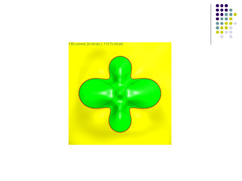
19. Experimental results Fitting unorganized data points without noise

20. Experimental results Fitting unorganized data points with noise

21. Experimental results Image contour detection

22. Conclusions and future work Dual evolution combines advantages of both parametric and implicit representations. The same evolution law and the synchronization step can produce the dual representations simultaneously and efficiently. Future work More complex topological changes (splitting + merging) Adaptive redistribution of control points during the evolution More intelligent and robust evolution speed function Other shape constraints (symmetries, convexity) Extend to 3D

23. References V. Caselles, R. Kimmel, and G. Sapiro, “Geodesic active contours”, International Journal of Computer Vision, 22(1), 1997, pp. 61-79 H. Pottmann, S. Leopoldseder and M. Hofer, “Approximation with Active B-spline curves and surfaces”, Proc. Pacific Graphics, 2002, pp. 8-25 W. Wang, H. Pottmann and Y. Liu, “Fitting B-spline curves to point clouds by squared distance minimization”, ACM Transactions on Graphics, to appear, 2005 T. W. Sederberg, J. Zheng, A. Bakenov and A. Nasri, “T-splines and T-NURCCS”, ACM Transactions on Graphics, 22(3), 2003, pp. 477- 484 J. Nocedal and S. J. Wright, “Numerical optimization”, Springer Verlag, 1999

24. Thanks!