1. University of Greenwich Business school
MSc in Financial Management and Investment Analysis

2. Economics for Finance and Investment Analysis

3. Doc. 7- Demand forecasting Dr M. Pourhosseini
October 2008
Doc. 7- Demand forecasting
Dr M. Pourhosseini

4. Demand management and forecasting
Doc 1, 2,3 explains in simple terms the relationships between supply and demand , elasticities and indifference curves.
In this lecture we discuss demand management and demand forecasting

5. Why do we need demand forecasting ?
to make good investment decision we need to:
assess the type and quantity of services required in advance .
Ensure efficient delivery on time
Provide right service levels to the right people when they want it
Determine cost-effective pricing
Allow rationing if required

6. Demand Management Resource Planning Production Planning Marketplace
Demand Mgt.
Master
Production
Planning

7. Basic Forecasting Approach
Understand the forecasting objective. What decisions will be made from the forecasts? What parties in the supply chain will be affected by the decision.
Integrate demand planning and forecasting. All planning activities within the supply chain that will use the forecast or influence demand should be linked.
Identify factors that influence the demand forecast. Is demand growing or declining? Is there are relationship (complementary or substitution) between products?

8. Forecasting Methods
Qualitative methods are subjective in nature since they rely on human judgment and opinion.
Quantitative methods use mathematical or simulation models based on historical demand or relationships between variables.

9. Forecasting Horizons.
Short Term (0 to 3 months): for inventory management and scheduling.
Medium Term (3 months to 2 years): for production planning, purchasing, and distribution.
Long Term (2 years and more): for capacity planning, facility location, and strategic planning.

10. Features of forecasts Forecasts are often not correct .
Every forecast should include an estimate of the forecast error.
The greater the degree of aggregation, the more accurate the forecast.
Long-term forecasts are usually less accurate than short-term forecasts.

11. Qualitative Forecasts
Survey Techniques
Planned Plant and Equipment Spending
Expected Sales and Inventory Changes
Consumers’ Expenditure Plans
Opinion Polls
Business Executives
Sales Force
Consumer Intentions

12. What are the Qualitative Methods
Jury of Executive Opinion (opinions of a small group of high-level managers is pooled).
Sales Force Composite (aggregation of salespersons estimate of sales in their territory).
Market Research Method (solicit input from customers or potential customers regarding future purchasing plans).
Delphi Method (a forecasting group uses a staff to prepare, distribute, collect, and summarize a series of questionnaires and survey results from geographically dispersed respondents, whose judgments are valued).

13. Quantitative Forecast Methods
Time Series Methods use historical data extrapolated into the future. These include :Moving averages, exponential smoothing methods, time series decomposition and Box-Jenkins Methods.
Causal Methods assume demand is highly correlated with certain environmental factors. Correlation methods and regression models
Simulation Methods imitate the consumer choices that give rise to demand to arrive at a forecast.

14. Regression analysis
Regression analysis is a useful tool to deal with the dependence one variable on other variables.
While a statistical relation in itself cannot logically imply causation. We can start by examining the strength or degree of linear association between two variables by considering the correlation coefficients between two variable

15. ECONOMETRIC TECHNIQUES-1
The discipline of econometrics is based on the idea that changes in economic activity are explained by a set of relationships between economic variables.

16. ECONOMETRIC TECHNIQUES -2
The “best mathematical arrangement” is called the
model which takes the form of an equation or
system of equations that describe the past
relationships according to economic theory and
statistical analysis.
The model is an abstraction of a real situation,
expressed in equation form and employed as a
forecasting tool to yield numerical results.

17. ECONOMETRIC TECHNIQUES-3
The construction a model is divided into three stages
planning,
development and
verification.

18. Types of Correlation Positive correlation Negative correlation
No correlation

19. Simple linear regression describes the
linear relationship between a predictor
variable, plotted on the x-axis, and a
response variable, plotted on the y-axis
dependent Variable (Y)
Independent Variable (X)

20. Y
1.0 X

21. Fitting data to a linear model
Observations are measure in a bivariate way
intercept
slope
residuals

22. Multiple regression
In demand analysis we can use regression analysis by distinguishing between dependent variable and explanatory variable in a two variable model. Or we can use a multiple regression model that has more than one explanatory or independent variable on the right hand side of the equation

23. ε Y ε X

24. Fitting data to a linear model
Observations are measure in a bivariate way
intercept
slope
residuals

25. How to fit data to a linear model?
The Ordinary Least Square Method (OLS)

26. Least Squares Regression
Model line:
Residual (ε) =
Sum of squares of residuals =
we must find values of and that minimise

27. Regression Coefficients

28. Required Statistics

29. Descriptive Statistics

30. Regression Statistics

31. explained by predictors
Variance to be
explained by predictors
(SST) Y

32. X1
Variance explained by X1
(SSR) Y
Variance NOT
explained by X1
(SSE)

33. Regression Statistics

34. Coefficient of Determination
Regression Statistics
Coefficient of Determination
to judge the adequacy of the regression model

35. Regression Statistics
Correlation
measures the strength of the linear association between two variables.

36. Regression Statistics
Standard Error for the regression model

37. The linear model with a single
predictor variable X can easily
be extended to two or more
predictor variables.

38. Partial Regression Coefficients
intercept
residuals
Partial Regression Coefficients (slopes): Regression coefficient of X after controlling for (holding all other predictors constant) influence of other variables from both X and Y.

39. Time Series Demand Model
Observed Demand = Systematic Component + Random Component.
Systematic Component measures the expected value of demand and consists of:
Level: the current deseasonalized demand.
Trend: the rate of growth or decline in demand.
Seasonality: the regular periodic oscillation in demand.
Random Component is that part of demand that follows no discernable or predictable pattern.The random component is estimated by the forecast error (forecast – actual demand).

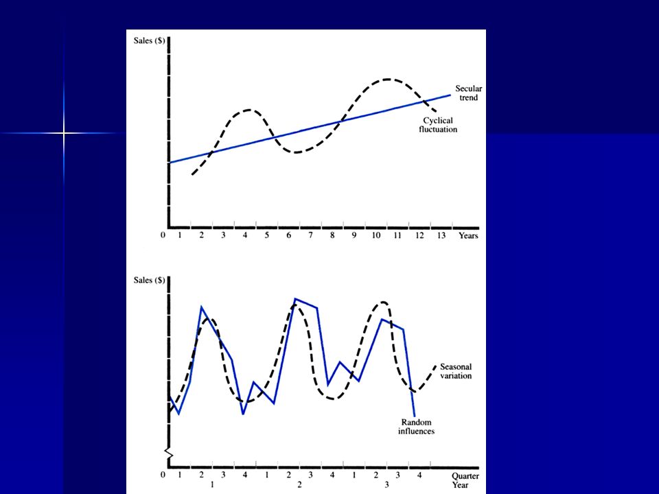
40. Time-Series Analysis Secular Trend Cyclical Fluctuations
Long-Run Increase or Decrease in Data
Cyclical Fluctuations
Long-Run Cycles of Expansion and Contraction
Seasonal Variation
Regularly Occurring Fluctuations
Irregular or Random Influences

42. Forecasting Approach (cont.)
Understand and Identify customer segments. Customer demand can be separately forecast for different segments based on service requirements, volume, order frequency, volatility, etc.
Determine the appropriate forecasting technique. Typically, using a combination of the different techniques is of the the most effective approach.
Establish performance and error measures. Forecasts need to be monitored for their accuracy and timeliness.

43. Would the future be like the past?
Regression analysis of time series data necessarily uses data from the past to quantify historical relationships.
If the future is like the past , then these historical relationships can be used to forecast the future.

44. What if the future is very different
But if the future differs fundamentally from the past , then those historical relationships might not be reliable guide to the future

45. Check if the time-series is stationary
We have to look at the data and find out if the past relationships in the time –series regression can be generalised to the future.
For this purpose we use the concept of stationarity.

46. Stochastic process
Stochastic come from the Greek word STOKHOS which means a target or bull’s eye
You throw darts at bull’s-eye on a dart board. Lucky to hit the bull’s eye only a few times , at other times the darts will be spread randomly around the bull’s -eye

47. What is stochastic process?
A stochastic process is a collection of random variables ordered in time.
A stochastic trend is a random movement of a variable over time

48. What is a realisation?
In the data you used for GDP in the workshop, you entered for 1977:1 a realisation.
In fact each observation is a realisation which is a random variable.

49. Realisation & stochastic process
The distinction between a realisation and a stochastic process is similar to the distinction between population and sample in cross-section al data
Just as we use sample data to draw inferences about a population , in time series we use the realisation to infer about stochastic process.

50. What is stationary stochastic process?
A process is said to be stationary if its:
Mean is constant over time
Variance is constant over time
The value of covariance between the two time period depends only on the distance between the two time periods and not the actual time at which the covariance is computed

51. STATIONARY TIME- SERIES PROPERTIES

52. is the covariance at lag k
is the covariance between two Y values k period apart
is the covariance between the values

53. If k=0 is simply the variance of Y

54. stationarity
Empirical work base on time series data assumes that the underlying time series is stationary
Some times Autocorrelation results because the time series in nonstationary
Or we might have spurious, nonsense regression despite having a very high R squared

55. Stationary time series
When the joint distribution of a time series and its lagged values does not change over time we can generalise past relationships to the future.
Before using a time-series regression, we have to check if it is stationary or not.

56. Why are stationary time-series so important?
Because if a time series is non-stationary ,we can study its behaviour only for the time period under consideration.
Each set of time series data will, therefore be for a particular episode.
It is not possible to generalize it to other time periods. For the purpose of forecasting ,such nonstationary time-series may be of little practical value.

57. Stationary times series

58. Characteristics of stationary time-series
In short, if a time-series is stationary ,its mean , variance and Autocovariance (at various lags)remain the same no matter at what point we measure them.
That is ,they are time invariant
Such time series will tend to return to its mean (called mean reversion)and fluctuations around the mean (measured by variance)will have a broadly constant amplitude

59. white noise process
A special type of stochastic process is called purely Random or white noise if it has:
Zero mean
Constant variance
Serially uncorrelated

60. Random Walk
Spurious regressions can arise if time series are not Stationary
Some financial time series exhibit Random Walk Phenomenon: the best prediction of price of a stock today is its price in the last trading day plus a purely random shock(error term)

61. Random walk without the drift
Suppose is a white noise error term with mean zero and constant variance. Then the series is said to be a random walk if
This model shows that the value of Y at the time t is equal to its value at time(t-1) plus a random shock; thus it is AR(1).

62. Random walk with a drift
Consider the following equation:
Where is the drift parameter. The name drift comes from the fact that
Drifts upward or downward depending on drift parameter, , being negative or positive.

63. Random walk models are nonstationary
In both models of random walk with or without drift ,the mean as well as variance increases over time, violating the conditions of stationarity.
A Random walk model, with or without drift, is a nonstationary stochastic process

64. The equation bellow is random walk

65. We face what is known as unit root problem, that is nonstationary.
The terms nonstationary , random walk and unit root can be treated as synonymous.

66. Nonstationary time series
The classical example of a non stationary time series is the random walk model.
The asset prices, such as stock prices or exchange rates follow a random walk : they are nonstationary
We have two types of random walk:
Random walk without drift(no constant or intercept term)
Random walk with drift (a constant term is present)

67. Problem with nonstationary series
In practice many economic time-series appear to be non-stationary.
If the time series variables are nonstationary , then one or more problems can arise :
The forecast can be biased
The forecast can be inefficient
Conventional OLS t-statistic can be misleading
For now , however , we simply assume that the series are jointly stationary and focus on regression with stationary variables

68. Stationary time-series
Stationary time -Series oscillates about a fixed mean value
Size of oscillations is approximately constant
Correlation between separated observation depends only on time distance between them
For AR(1) model, can show that Xt is stationary if
-1 < b < 1

69. Sources of nonstationarity
Precisely which of these problems occurs, and its remedy depends on the source of stationarity.
We will study the problems posed by, tests for and solutions to two empirically important types of stationarity in economic time series, trends and breaks in coming weeks.

70. b = 0: Xt is a completely random series

71. b = 0.7: Xt is a stationary series

72. b = -0.3: Xt is a stationary series

73. b = 1.2: Xt “Explodes”

74. b = 1: Xt is a non-stationary series Random Walk
series has “unit root” (b = 1)

75. What will happen if the series is nonstationary?
Forecasting will be meaningless if underlying time series are non stationary
Causality tests assume time series data are stationary, therefore stationarity should precede tests of causality

76. Unit root stochastic process
If a series has a unit root ,then it is non stationary.
In practice , it is important to find out a time series is stationary or not by having a unit root test

77. What is Autoregressive Distributed Lag (ADL) model ?
Economic theory often suggests more variables can be added to the model to produce a time series model with multiple predictors.
When other variables and their lags are added to an autoregression, the result is an Autoregressive Distributed Lag (ADL) model

78. Nonstationarity tests
In the next lecture we will learn about different unit root tests.
One of these tests has been developed by two econometricians D.A. Dickey and W.A. Fuller
The usual t student test is not valid if the series is nonstationary. That is, it does not have an asymptotic normal distribution
Dickey and Fuller have estimated the appropriate critical values for the unit root test.

79. Autoregression : AR (1)
AR (1), is a regression model that relates a time series variable to its immediate past value.s

80. AR (2)
AR (2), is a regression model that relates a time series variable to its immediate past value and the time t-2.
AR (4), is a regression model that relates a time series variable to its immediate past value , the time t-2 , the time t-3 and the time t-4.

81. How can we use regression model and time series analysis in forecasting ?
We can develop models that relate quantity demanded to price and elasticities.
We can for example study a model for energy demand
First we need to specify a model in a functional form

82. * quality demanded (yd) and price (x)
Economic Models
Demand Models
* quality demanded (yd) and price (x)
* constant elasticity
ln(yt )= 1 + 2ln(x)t + et d

83. Log-Log (Constant Elasticity Model)
Useful Functional Forms
Log-Log (Constant Elasticity Model)
ln(yt)= 1 + 2ln(xt) + et yt
slope: 2 elasticity: 2 xt

84. Log-Log Models y x

85. Log-Log Models y x

86. Demand for Energy
In the next lecture , see Doc 10 we develop a model describing demand for energy by considering the requirements of consumers and producers