1. Chapter 5 Hypothesis Testing

2. 5.1 - Introduction Definition 5.1.1 Hypothesis testing is a formal approach for determining if data from a sample support a claim about a population. 1.State the null and alternative hypotheses 2.Calculate the test statistic 3.Find the critical value (or calculate the P-value) 4.State the technical conclusion 5.State the final conclusion

3. The Process Claim: More than half the students at a particular university are from out of state Step 1: State the null and alternative hypotheses – Define the parameter p = The proportion of all students at the university who are from out of state – State the hypotheses H 0 : p = 0.50 H 1 : p > 0.50

4. The Process

5. Step 3: Find the critical value – At the 95% confidence level,

6. The Process Step 4: State the technical conclusion – One of two statements: Reject H 0 or Do not reject H 0 – Reject H 0 if the test statistic falls into the critical region and do not reject H 0 otherwise – z = 2.36, critical region: [1.645, ∞) Reject H 0

7. The Process Step 5: State the final conclusion – The data support the claim

8. P-value Method Criteria 1.Reject H 0 if P-value ≤ α 2.Do not reject H 0 if P-value > α

9. P-value Method

10. 5.2 – Testing Claims about a Proportion

11. 1-Proportion Z-Test The test statistic is The critical value is a z-score and the P-value is an area under the standard normal density curve.

12. 1-Proportion Z-Test

13. Example 5.2.1 A student claims that less than 25% of plain M&M candies are red. A random sample of 195 candies contains 37 red candies. Use this data to test the claim at the 0.05 significance level. 1.The parameter about which the claim is made is p = The proportion of all M&M candies that are red

14. Example 5.2.1

16. Types of Errors

17. 5.3 – Testing Claims about a Mean

18. T-Test Requirements 1.The sample is random 2.Either the population is normally distributed or n > 30

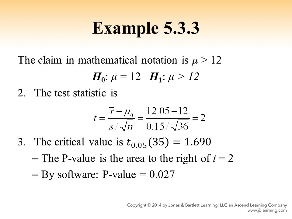
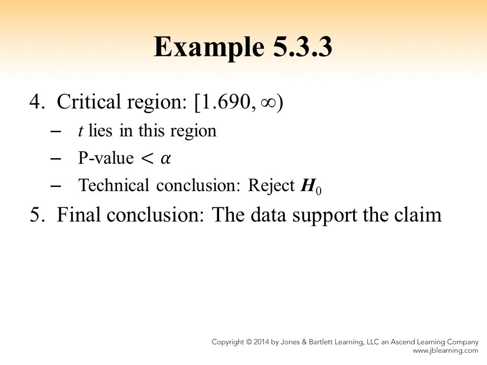
19. Example 5.3.3

22. 5.4 – Comparing Two Proportions

23. 2-Proportion Z-Test Requirements 1.Both samples are random and independent 2.In both samples, the conditions for a binomial distribution are satisfied 3.In both samples, there are at least 5 successes and 5 failures

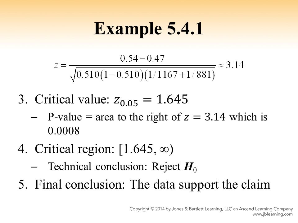
24. Example 5.4.1 In a survey of voters in the 2008 Texas Democrat primary, 54% of the 1167 females voted for Hillary Clinton while 47% of the 881 males voted for Clinton (data from www.CNNPolitics.com, March 5, 2008). Use this data to test the claim that of the voters in the 2008 Texas Democrat primary, the proportion of females who voted for Clinton is higher than the proportionof males who voted for Clinton. www.CNNPolitics.com

25. Example 5.4.1

27. 5.5 – Comparing Two Variances

28. F-Test

29. Example 5.5.1

30. 1.The parameters about which the claim is made are 2.Test statistic:

31. Example 5.5.1

32. 5.6 – Comparing Two Means

33. Equal Population Variances

34. Unequal Population Variances Test statistic: The critical value is a t-score with r degrees of freedom where r is If r is not an integer, then round it down to the nearest whole number

35. Requirements 1.Both samples are random 2.The samples are independent 3.Both populations are normally distributed or both sample sizes are greater than 30

36. Example 5.6.1

37. 1.The parameters about which the claim is made are 2.Assume equal population variances. Test statistic:

38. Example 5.6.1

39. Paired T-Test

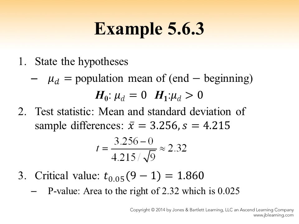
40. Example 5.6.3 At a large university, freshman students are required to take an introduction to writing class. Students are given a survey on their attitudes toward writing at the beginning and end of the class. Each student receives a score between 0 and 100 (the higher the score, the more favorable his or her attitude toward writing). Test the claim that the scores improve from the beginning to the end.

41. Example 5.6.3

43. 4.Critical region: [1.860, ∞) – Reject H 0 5.Final conclusion: The data support the claim

44. 5.7 – Goodness-of-fit Test

45. Chi-square Goodness-of-fit Test

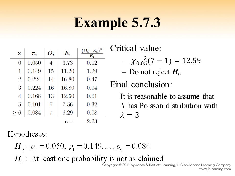
46. Example 5.7.3 A student simulated dandelions in a lawn by randomly placing 300 dots on a piece of paper with an area of 100 in 2. He then randomly chose 75 different 1 in 2 sections of paper and counted the number of dots in each section.

47. Example 5.7.3

49. 5.8 – Test of Independence Two students want to determine if their university men’s basketball team benefits from home-court advantage. They randomly select 205 games played by the team and record if each one was played at home or away and if the team won or lost (data collected by Emily Hudgins and Courtney Santistevan, 2009). “Contingency Table”

50. Chi-square Test of Independence

51. Test of Independence

52. Example

53. 5.9 – One-way ANOVA A seed company plants four types of new corn seed on several plots of land and records the yield (in bushels/acre) of each plot as shown below. Test the claim that the four types of seed produce the same mean yield.

54. One-way ANOVA

56. Example 5.9.3

57. 5.10 – Two-way ANOVA Randomized Block Design A statistics professor is comparing four different delivery methods for her introduction to statistics class: face-to- face, online, hybrid, and video (called the treatments). – She divides the population of students into three groups according to their overall GPA: high, middle, and low. (called blocks) – She randomly chooses four students from each block and randomly assigns each one to a class using one of the delivery methods – At the end of the semester she records each student’s overall grade

58. Two-way ANOVA Two questions: 1.Do the four treatments have the same population mean? 2.Do the blocks have any affect on the scores?

59. Two-way ANOVA

60. ANOVA Table P-value = 0.271 – Do not reject H 0 – There is not a statistically significant difference between the treatment means P-value = 0.008 – Reject H B – There is a statistically significant difference in the block effects

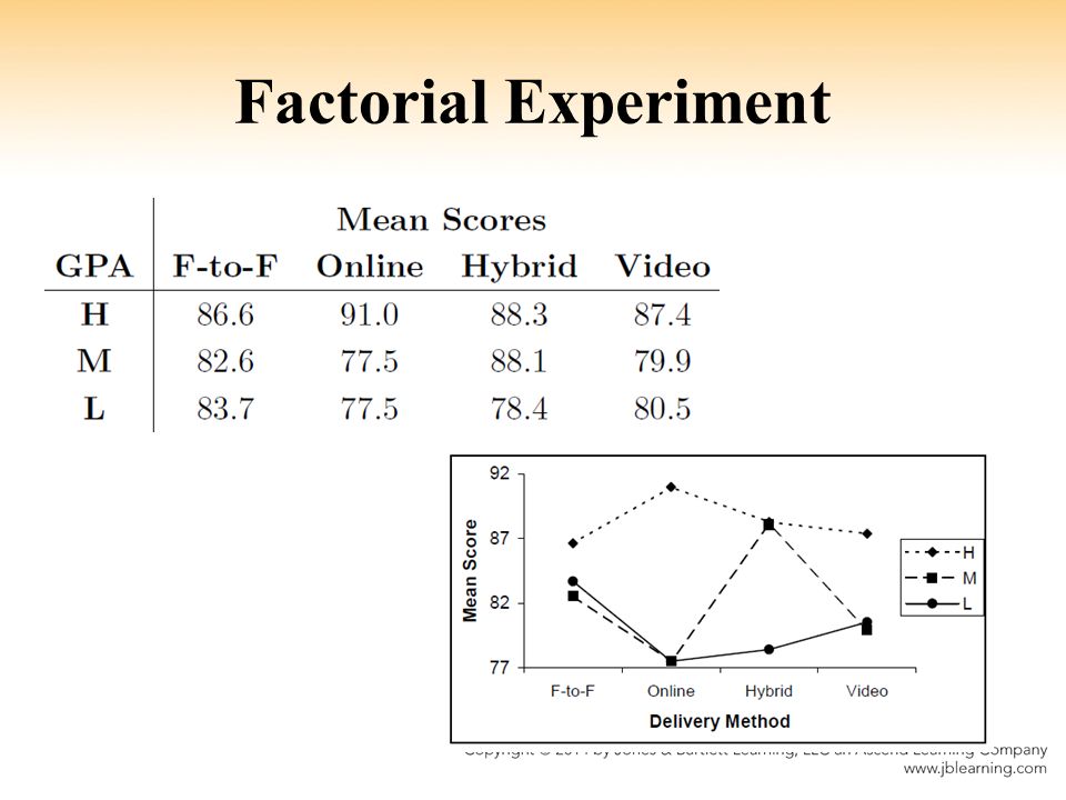
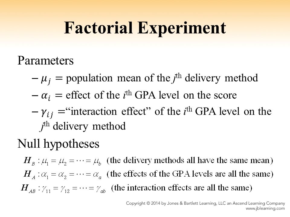
61. Factorial Experiment The statistics professors randomly chooses 16 students from each GPA level, randomly assigns four to each delivery method, and records their scores at the end of the semester. Three questions: 1.Is there any difference between the population mean scores of the delivery methods? 2.Does the GPA level affect the scores? 3.Does the interaction of the delivery method and GPA level affect the scores?

62. Factorial Experiment

65. ANOVA Table P-value = 0.176 – Do not reject H B – There is not a statistically significant difference between the means of the delivery methods P-value = 0.000 – Reject H A – There is a statistically significant difference in the effects of the GPA levels

66. ANOVA Table P-value = 0.004 – Reject H AB – There is a statistically significant difference in the interaction effects Overall – There is not a “best” method – Consider certain delivery methods to certain GPA levels