Download presentation
Presentation is loading. Please wait.

1
Chapter 3 Binary Image Analysis

2
Types of images ► Digital image = I[r][c] is discrete for I, r, and c. B[r][c] = binary image - range of I is in {0,1} B’[r][c] – complement or inverse of B = 1 if B[r][c]=0 = 0 if B[r][c]=1 Gray-scale image = range of I is in {min, min+1,…,max-1,max} Multispectral image = vector-valued ► Ex. Color image = range is in { | (r,g,b) in {0,1,…,max} }
![Types of images ► Digital image = I[r][c] is discrete for I, r, and c.](http://images.slideplayer.com/22/6345075/slides/slide_2.jpg " B[r][c] = binary image - range of I is in {0,1} B’[r][c] – complement or inverse of B = 1 if B[r][c]=0 = 0 if B[r][c]=1 Gray-scale image = range of I is in {min, min+1,…,max-1,max} Multispectral image = vector-valued ► Ex. Color image = range is in { | (r,g,b) in {0,1,…,max} }.")
3
How do we create binary images? ► By selecting (foreground) pixels of interest and thereby separating them from background pixels = segmentation Ex. Thresholding = selecting ranges of gray (or color) values ► Ex. 1 if value>100 0 otherwise 0 = background 1 = foreground
 pixels of interest and thereby separating them from background pixels = segmentation Ex. Thresholding = selecting ranges of gray (or color) values ► Ex. 1 if value>100 0 otherwise 0 = background 1 = foreground.")
8
Pixel and its neighbors ► 4-neighbors/4-adjacent/4-connected {,,, } Or as displacements: ► {,,, } ► How about 8-adjacent? Distances?

9
Masks

10
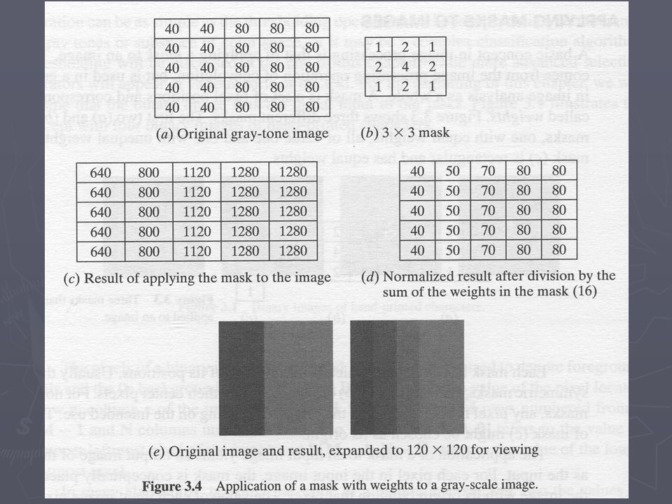
► Mask = set of pixel positions and corresponding values called weights ► Mask origin = usually center ► How? 1.Calculate sum of products ► Boundary 1.Replicate nearest pixel value 2.Use 0 2.Normalize (or an amplitude shift will occur) Applying masks to images
 Applying masks to images.")
11
► Derived from convolution: ► Discrete form is cross correlation: ► where f is the input image, h is the mask/filter kernel, and g is the output image result

12
Convolution ► See http://en.wikipedia.org/wiki/Convolution for some nice animations. http://en.wikipedia.org/wiki/Convolution
14
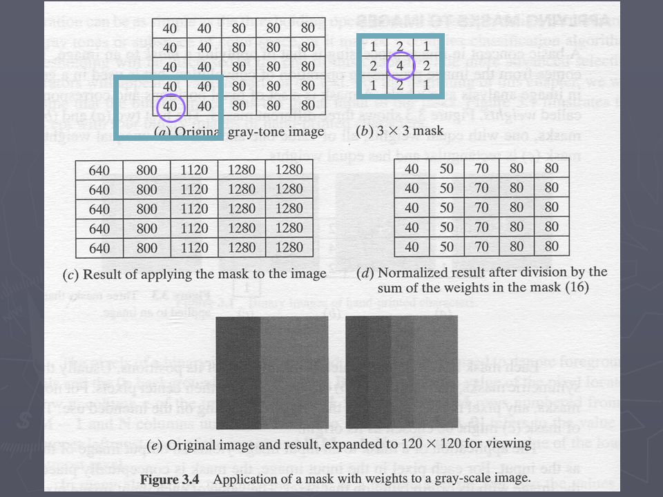
1*40+2*40+1*80+ 2*40+4*40+2*80+ 1*40+2*40+1*80 =800

15
1*40+2*80+1*80+ 2*40+4*80+2*80+ 1*40+2*80+1*80 =1120

16
But what about borders? ► When we are missing data at the edges, we typically do one of the following: 1.Copy to the missing value, the nearest neighboring value. 2.Use 0 for the missing value(s). (Regardless, it really doesn’t matter, but we need to consistently do something.)
. (Regardless, it really doesn’t matter, but we need to consistently do something.).")
18
1*40+2*40+1*40+ 2*40+4*40+2*40+ 1*40+2*40+1*40 =640 Method 1: copy nearest

19
The importance of normalizing the result. ► Otherwise, the values might get larger and larger (brighter and brighter).
..")
20
1+2+1+ 2+4+2+ 1+2+1 =16 640/16

21
1 2 1 2 4 2 1 2 1

22
Counting objects (instead of holes) ► If we complement our masks from the hole counting algorithm, we can count objects! ► (Or if we complement our image, we can count objects!)
.")
23
I don’t care for this format!

24
Object counting assumptions (complement of hole counting assumptions) 1. All image border pixels must be 0s. 2. Each region of 1s (objects) must be 4- connected. 3. Objects must also be simply connected (not contain any holes).
 must be 4- connected. 3. Objects must also be simply connected (not contain any holes)..")
25
Implement object counting algorithm ► Check assumptions 1 and 2. (Skip 3 for now.) ► Report number of objects. ► Exercise 3.1 p. 56 - Efficiency of counting objects. What is the maximum number of times that the function count_objects examines each pixel of the image? How can functions external_match and internal_match be coded to be as efficient as possibly?
 ► Report number of objects. ► Exercise 3.1 p Efficiency of counting objects. What is the maximum number of times that the function count_objects examines each pixel of the image. How can functions external_match and internal_match be coded to be as efficient as possibly .")
26
More object analysis ► So far, we can count objects! But how big are they? What shape are they?

27
Paths There exists a path from (x 1,y 1 ) to (x n,y n ) iff there exists a sequence (x 1,y 1 ), (x 2,y 2 ), …, (x n,y n ) s.t. all (x i,y i ) and (x i+1,y i+1 ) are (4- or 8-) connected and B(x i,y i )=B(x i+1,y i+1 ).
 and (x i+1,y i+1 ) are (4- or 8-) connected and B(x i,y i )=B(x i+1,y i+1 )..")
28
Connected component A connected component of value v is a set of pixels C with: 1.each having value v 2.and for every c and d in C, there exists a path from c to d.

29
Objects are 1s (and white) here.
 here.")
30
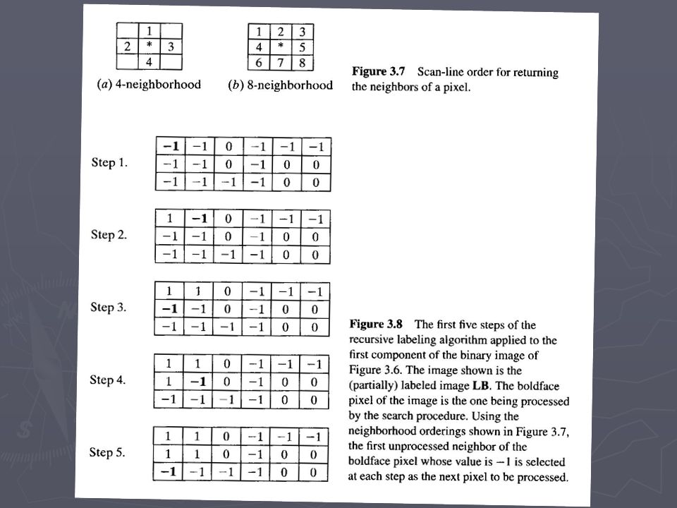
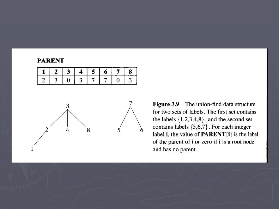
Labels ► 0 = background (not part of any object) ► 1 = first labeled object ► 2 = second labeled object ► … ► -1 = part of an unlabeled object (ready for labeling)
 ► 1 = first labeled object ► 2 = second labeled object ► … ► -1 = part of an unlabeled object (ready for labeling)")
31
I don’t care for this format! Recursive connected components algorithm: 3 functions

32
I don’t care for this format! Recursive connected components algorithm // 0 --> 0; 1 --> -1 // incremented before use so first will actually be 1

33
I don’t care for this format! Recursive connected components algorithm (Why not use r and c instead of L and P, respectively?)
.")
34
I don’t care for this format! Recursive connected components algorithm <-- What does this mean/do? <-- recursion! This is an example of a flood fill algorithm (see http://en.wikipedia.org/wiki/Flood_fill for nice animations). http://en.wikipedia.org/wiki/Flood_fill
.")
35
Begin skip other algorithms in this section.

44
End skip.

Similar presentations


 Automatic Perception 12+15 Volker Krüger Aalborg Media Lab Aalborg University Copenhagen>")

 –division or separation of the image into segments (connected regions) of similar properties.>")
 to binary (1 bit/pixel)>")


