1. Economic History (Master PPD & APE, Paris School of Economics) Thomas Piketty Academic year 2015-2016 Lecture 2: The dynamics of capital accumulation: private vs public capital and the Great Transformation (Tuesday September 15 th 2015) (check on line for updated versions)on line

2. The very long-run: Britain and France 1700-2010 Long tradition of national wealth estimates in Britain and France in the 18th-19th centuries: Britain: Petty, King, Giffen, etc.; France: Vauban, Lavoisier, Colson, etc. National balance sheets: estimates of all assets and liabilities held by residents of a country (and by the government) (« Bilans patrimoniaux par pays ») These estimates are not sufficientely precise to study short-run fluctuations; but they are fine to study broad orders of magnitudes and long-run evolutions See « Capital is Back – Wealth-Income Ratios in Rich Countries 1700-2010 », 2013, Data Appendix, Database, for detailed bibliography and methodological issuesData AppendixDatabase

3. Longest series: Britain and France national wealth/national income ratio β n =W n /Y over 1700-2010 National wealth W n = Private wealth W + Public (or government) wealth W g W n = Domestic capital K + Net foreign assets NFA Domestic capital K = agricultural land + residential housing + other domestic k (=offices, structures, machines, patents, etc. used by firms and administrations) Two major facts: (1) huge U-shaped curve: β n ≈700% over 1700-1910, down to 200-300% around 1950, up to 500- 600% in 2000-2010 (2) Radical change in the nature of wealth (agricultural land has been gradually replaced by housing, business and financial capital), but total value of wealth did not change much in the very long run

6. The rise and fall of foreign assets NFA close to 0 in 1700-1800 and 1950-2010, but very large in 1870-1910 = the height of the « first globalization » and of colonial empires In 1910, NFA≈200% of Y in UK, ≈100% in France These enormous net foreign assets disappeared between 1910 and 1950 and never reappeared (but large cross-border gross positions developed since 1970s-80s: « second globalization ») 2010: Y ≈ 30 000€, W n ≈ 180 000€ (β n ≈ 6), including 90 000€ in housing and 90 000€ in other domestic k (financial assets invested in firms and govt) 1700: assume Y ≈ 30 000€, then W n ≈ 210 000€ (β n ≈ 7), including 150 000€ in agricultural land and 60 000€ in housing and other domestic capital 1910 (UK): assume Y ≈ 30 000€, then W n ≈ 210 000€ (β n ≈ 7), including 60 000€ in housing, 90 000€ in other domestic capital and 60 000€ in net foreign assets

7. With NFA as large as 100-200% Y, the net foreign capital income is very large: around 1900-1910, as large as 5% Y in France and 10% Y in Britain (average rate of return r=5%) In effect, both countries were able to have permanent trade deficits (about 2% Y in 1870-1910) and still to have a current account surplus and to accumulate more foreign reserves; i.e. they were consuming more than they what were producing, and at the same time they were getting richer Two conclusions: (1) it’s nice to be a owner; (2) there’s no point accumulating trade surpluses for ever

8. Private versus public wealth National wealth W n = Private wealth W + Public wealth W g Private wealth = private assets – private debt Public wealth = public assets – public debt Today, in most rich countries, public wealth close to 0 (public assets ≈ public debt ≈ 100% Y), and private wealth ≈ 95-100% of national wealth But it has not always been like this: sometime the govt owns a significant part of national wealth (20-30% in 1950s-60s in W. Europe; 80% in USSR); sometime govt wealth<0 (huge debt), so that private wealth is significantly larger than national wealth

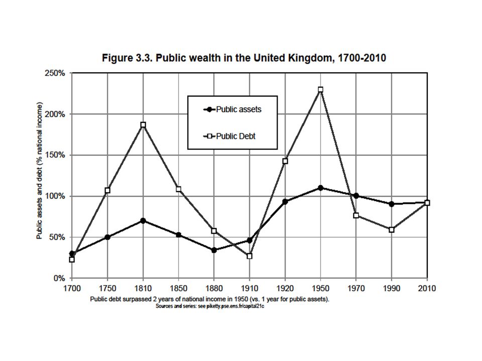
10. Britain: public debt and Ricardian equivalence Britain = the country with the longest historical episodes of public debt: about 200% of Y around 1810- 1820 (it took a century to reduce it below 50% by 1910, after a century of budget surpluses), and about 200% of Y again around 1950 (it was reduced faster, thanks to inflation) Big difference with France (large inflation and/or repudiation during 1790s & World Wars 1 and 2) and Germany (the country with the largest inflation in 1910-1950, even excluding 1924) Britain always paid back its debt (limited inflation, except 1950-1980); this is why it took so long to reduce debt, especially during 19c

14. Q.: What is the impact of public debt on capital accumulation? A.: It depends on how the private saving responds to public deficit National saving S n = private saving S + public saving S g (<0 if public deficit) Suppose dS g <0 (public deficit↑) If dS=0 (no private saving response), then dS n <0 → decline in national wealth W n : in effect public deficits absorb part of private saving (=« crowding out ») But if dS>0, i.e. private saving increase in order to absorb the extra deficit, then crowding-out might be limited In case dS=-dS g, then dS n =0: national saving and national wealth are unaffected by public deficit = apparently what happened in UK 1810-1830: huge public debt, but no decline in private investment; extra private saving by British wealth holders, so that we observe a rise in private wealth, and no decline in national wealth = what Ricardo observes in 1817

16. Key question: why was there no crowding out? Barro 1974: in a representative agent model, rational agents should anticipate that they will pay more taxes in the future if today’s public deficit increase, so they save more in order to make reserves (for themselves or their successors) so as to pay these taxes in the future → the timing of taxes is irrelevant, « debt neutrality » (see also Barro 1987, Clark 2001) Barro 1974Barro 1987Clark 2001 Pb: it is unclear whether the representative agent model makes sense to study these issues; in 19c Britain, the agents holding public debt (=top 1% or top 10% wealth holders) are not the same as those paying taxes (=the entire population) Public debt always involves large transfers between income groups: for high wealth agents, it is better to lend money than to pay taxes… as long as the debt is paid back = big difference between 19c and 20c; will 21c be more like 19c, i.e. debt will be paid back? Whether the Ricardian equivalence holds depends on the prosperity of private savers, the rate of return that they are being offered, the ability of the govt to convince them that they will be paid back; in 19c UK, r was high, and govt highly credible

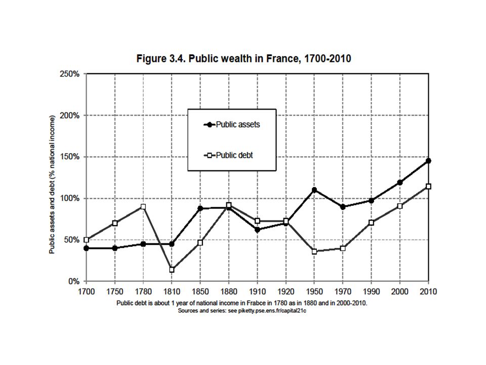
17. France: a mixed economy in 1950-1980 Historically, high public debt in France was always inflated away (more difficult with €) In 1950, public debt 120% Y (public buildings + nationalized firms), so that net public wealth close to 100% Y; given that private wealth was close to 200% Y at that time, this means that in effect the govt owned about 1/3 of national wealth (and over 2/3 of large companies) Same pattern in Germany 1950 (and Britain 1970) = the postwar mixed economy Rise in public debt + privatization of public assets played a big role in rise of private wealth since 1980 (see next lecture)

19. Capital in Germany Same general pattern as in Britain and France Except that NFA smaller in Germany in 1870- 1910 (no colonial empire, late industrialization) Except that the level of β n is lower in Germany during 1950-2010 period: lower real estate prices, lower stock market prices (stakeholder capitalism?) Except that NFA has been rising a lot in 1990s- 2000s

25. Capital in America Very different historical pattern than in Europe Rising β n during 19c, almost stable in 20c Level of β n generally smaller than in Europe, particularly in 19c Two factors: less time to accumulate capital; lower land price (more land in volume, but less land in value) NFA always close to 0 in US; but <0 in Canada

30. Capital and slavery in the US In the US 1770-1865, market value of slaves ≈ 150% of Y ≈ as much as agricultural land In Southern US, slaves ≈ 300% of Y, so that total private wealth (incl.slaves) = as large as in Europe Huge historical literature on US slavery system: Fogel, etc. (see Data Appendix)Data Appendix See also recent research on compensation to slave owners after the abolition of slavery in Britain 1833 (see UCL project) and France (Haiti debt 1825) (see also Graeber, Debt – The first 5000 years)UCL project

33. On the value of human capital Extreme case: if a tiny fraction owns the rest of the population, then the value of slaves (=human capital) can be much larger than non- human capital Simple computation: assume marginal products of capital and labor are such as capital share = α (= r β) and labor share = 1-α (Cobb-Douglas production function: Y=F(K,L)=K α L 1-α ); if future labor income flows are capitalized at the same rate r, then the value of human capital should be = (1-α)/r (more on this: see lectures 3-4) If α=30%, 1-α=70%, r=5%, then market value of (non-human) capital = α/r = 600%, and market value of human capital (slaves) = 1400%; total capital = 2000% (=1/r) I.e. the market value of human k has always been higher than the market value of non-human k, simply because labor share >50% But outside slave societies, it really does not make much sense to compute a market value of human capital: in modern legal systems, one cannot sell one’s labor force on a permanent basis

34. Summing up: what have we learned? National wealth-income ratios β n =W n /Y followed a large U-shaped curve in Europe: 600-700% in 18c-19c until 1910, down to 200-300% around 1950, back to 500-600% in 2010 U-shaped curve much less marked in the US Most of the long run changes in β n are due to changes in the private wealth-income ratios β=W/Y But changes in public wealth-income ratios β g =W g /Y (>0 or <0) also played an important role (e.g. amplified the β decline between 1910 and 1950) Changes in net foreign assets NFA (>0 or <0) also played an important role (e.g. account for a large part of the β decline between 1910 and 1950)

37. Let’s move to theory: how can we explain capital-income ratios β=W/Y ? We first need a theory of why people own wealth: if economic agents only care about current consumption, then they should not own any wealth, i.e. β=0. So we need a dynamic model (at least two periods) where agents care about the future. OLG model: agents maximize U(c t,c t+1 ), where c t = young-age consumption (working age) & c t+1 = old-age consumption Depending on utility function U(.,.) (rate of time preference, etc.), demographic parameters, etc., one obtains different saving rates and long run β (see « Modigliani triangle » formula in lecture 6) Pb with the pure life-cycle model: individuals are supposed to die with zero wealth; in the real world, inherited wealth is also important Models with utility for bequest: U(c t,w t+1 ), where c t = lifetime consumption (young + old) & w t+1 = bequest (wealth) left to next generation Depending on the strength of the bequest motive in utility function U(c,w), one can obtain any saving rate and long run β

38. Harrod-Domar-Solow formula: β=s/g Exemple: if agents maximize U(c t,Δw t =w t+1 -w t ), then with U(c,Δ)=c 1-s Δ s, we get a fixed saving rate s t =s, and β t → β = s/g (i.e. Max U(c t,Δw t ) under c t +Δw t ≤y t → Δw t = s y t ) More generally, this is what we get in any one-good capital accumulation model, whatever the saving motives and utility fonctions behind the saving rate s t : I.e. assume that: W t+1 = W t + s t Y t → dividing both sides by Y t+1, we get: β t+1 = β t (1+g wt )/(1+g t ) With 1+g wt = 1+s t /β t = saving-induced wealth growth rate 1+g t = Y t+1 /Y t = total income growth rate (productivity+population) If saving rate s t → s and growth rate g t → g, then: β t → β = s/g Exemple: if s=10%, g=2%, β t → β = 500% This is a pure accounting identity: β = 500% is the only wealth-income ratio such that a saving rate of 10% of income corresponds to a growth rate of 2% of the capital stock Intuition: the more you save, the more you accumulate, especially in a slow- growth economy (on these models, see Piketty-Zucman 2013 section 3)Piketty-Zucman 2013 section 3

39. Another special case: the dynastic model Pure dynastic model = model with infinite horizon and fixed rate of time preference = individuals behave as if they were infinitely lived Discrete time version: U t = ∑ t≥0 U(c t )/(1+θ) t (θ = rate of time preference) Budget constraint: ∑ t≥0 c t /(1+r) t ≤ ∑ t≥0 y t /(1+r) t r t = rate of return = = f’(k t ) = borrowing interest rate (perfect capital markets) Closed economy, representative agent: ind. wealth w t = per capita capital stock k t First-order condition: U’(c t+1 )/U’(c t )=(1+θ)/(1+r) Assume U(c)= c 1- γ /(1- γ ), i.e. U’(c)= c - γ, (U(c)=log(c) if γ=1) FO condition: c t+1 =c t [(1+r)/(1+θ)] 1/ γ Intuition: if r > θ, then agents want to postpone consumption to the future (conversely if r < θ), and all the more so if γ close to 0, i.e. U(c) close to linear γ = curvature of U(c) (risk aversion coefficient), 1/ γ = intertemporal elasticity of substitution Steady-state growth path: y t = y 0 (1+g) t, k t = k 0 (1+g) t, c t = c 0 (1+g) t → 1+r = (1+θ) x (1+g) γ (with continuous time: r = θ + γ g ) → if g=0, then r=θ (>g) : rate of return is entirely determined by preferences

40. With Cobb-Douglas production function y=f(k)=k α, then r=f’(k)=αk α-1, so that capital income rk=αy, i.e. capital-income ratio β=k/y= α/r I.e. if r = θ + γ g, then β=α/(θ + γ g) Exemple: if g=0, θ=5% and α=25%, then β= α/θ =500% I.e. if lower θ (more patient), higher β In effect, in the dynastic model, agents save a fraction g/r of their capital income rk, so that their wealth rises at rate g, like the rest of the economy (i.e. with g=1% and r=5%, they save 1/5=20% of their capital income, and eat the rest → saving rate s = α g/r capital-income ratio β = s/g= α/r =g=0 = special case of Harrod-Domar-Solow formula

41. Inequality in the dynastic model For simplicity, assume a two-point distribution of wealth. Dynasties can be of one of two types: either they own a large capital stock k t A, or they own a low capital stock k t B (with k t A > k t B ). The proportion of high-wealth dynasties is equal to λ (and the proportion of low- wealth dynasties is equal to 1-λ), so that the average capital stock in the economy k t is given by: k t = λk t A + (1-λ)k t B Result: any distribution such that the average wealth k* satisfies f’(k*)=r= θ + γ g can be a steady-state I.e. any wealth inequality is self-sustaining, both within countries and between countries, including with negative wealth k t B <0 for the poor (possibly extreme negative wealth = slavery) With shocks and mobility, steady-state wealth inequality is a rising function of the differential r-g (see lecture 6)

42. To summarize: Harrod-Domar-Solow formula β = s/g is a pure accounting formula and is valid with any saving motive and utility function Wealth increase in the utility function: Max U(c t,Δw t =w t+1 -w t ) → if U(c,Δ)=c 1-s Δ s, then fixed saving rate s t =s, β t → β = s/g (i.e. Max U(c t,Δw t ) under c t +Δw t ≤y t → Δw t = s y t ) Total wealth or bequest in the utility function: Max U(c t,w t+1 ) → if U(c,w)=c 1-s w s, then w t+1 =s(w t + y t ), β t → β = s/(g+1-s) = s’/g (with s’=s(1+β)-β = corresponding saving rate out of income) Pure OLG lifecycle model: saving rate s determined by demographic structure (more time in retirement → higher s), then β t → β = s/g Dynastic utility: Max Σ U(c t )/(1+θ) t, with U(c)=c 1-1/ γ /(1-1/ γ ) → unique long rate rate of return r t → r = θ + γ g > g → long run saving rate s t → s = αg/r, β t → β = α/r = s/g (on these models, see Piketty-Zucman 2013 section 3)Piketty-Zucman 2013 section 3

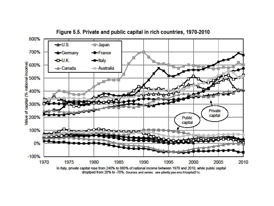
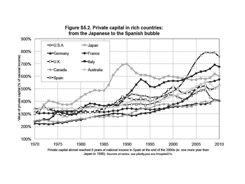
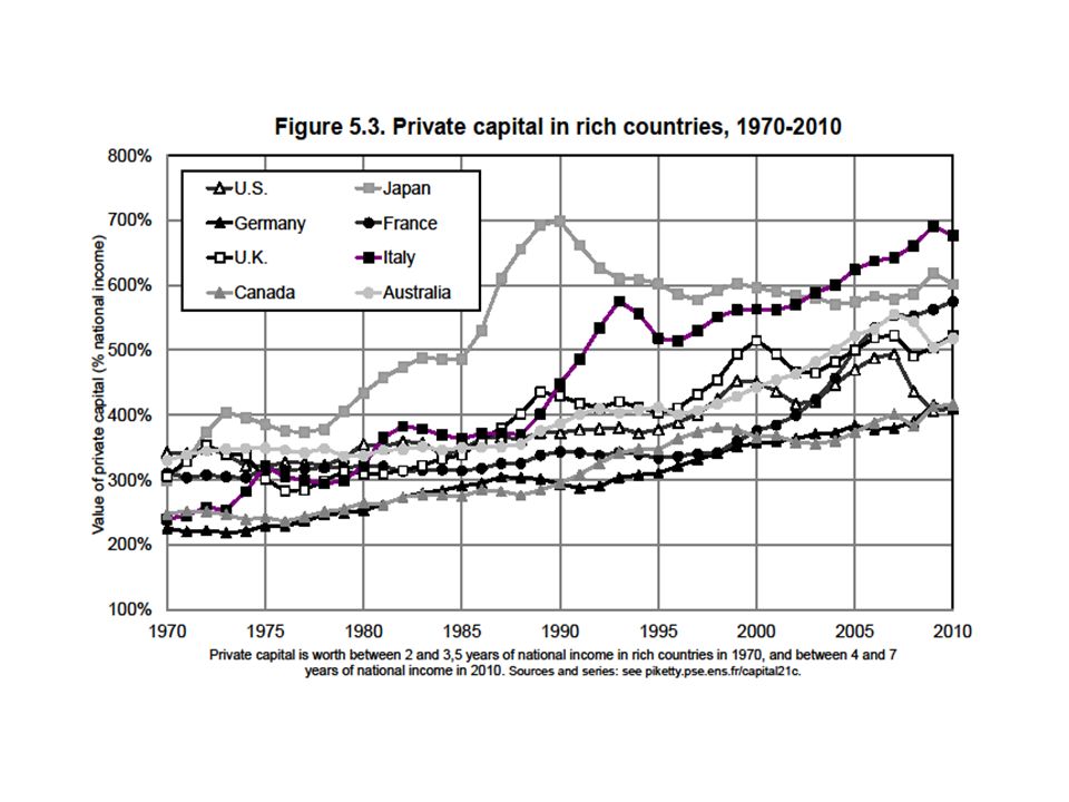
43. The rise of wealth-income ratios in rich countries 1970-2010: volume or price effects ? Over 1970-2010 period, the analysis can be extented to top 8 developed economies: US, Japan, Germany, France, UK, Italy, Canada, Australia Around 1970, β≈200-350% in all rich countries Around 2010, β≈400-700% in all rich countries Asset price bubbles (real estate and/or stock market) are important in the short-run and medium-run But the long-run evolution over 1970-2010 is more than a bubble: it happens in every rich country, and it is also consistent with the basic theoretical model β=s/g

45. The rise of β would be even larger is we were to divide private wealth W by disposable household income Y h rather than by national income Y Y h used to be ≈90% of Y until early 20c (=very low taxes and govt spendings); it is now ≈70-80% of Y (=rise of in-kind transfers in education and healh) β h =W/Y h is now as large as 800-900% in some countries (Italy, Japan, France…) But in order to make either cross-country or time- series comparisons, it is better to use national income Y as a denominator (=more comprehensive and comparable income concept)

47. 1970-2010: rise of private wealth-income ratio β, decline in public wealth-inccome ratio β g But the rise in β was much bigger than the decline in β g, so that national wealth-income ratio β n =β+β g rose substantially Exemple: Italy. β rose from 240% to 680%, β g declined from 20% to -70%, so that β n rose from 260% to 610%. I.e. at most 1/4 of total increase in β can be attributed to a transfer from public to private wealth (privatisation and public debt).

49. In most countries, NFA ≈ 0, so rise in national wealth-income ratio ≈ rise in domestic capital-output ratio; in Japan and Germany, a non-trivial part of the rise in β n was invested abroad (≈ 1/4)

51. Main explanation for rise in wealth-income ratio in the very long run: growth slowdown and β = s/g (Harrod-Domar-Solow steady-state formula) One-good capital accumulation model: W t+1 = W t + s t Y t → dividing both sides by Y t+1, we get: β t+1 = β t (1+g wt )/(1+g t ) With 1+g wt = 1+s t /β t = saving-induced wealth growth rate 1+g t = Y t+1 /Y t = total income growth rate (productivity+population) If saving rate s t → s and growth rate g t → g, then: β t → β = s/g E.g. if s=10% & g=2%, then β = 500%: this is the only wealth-income ratio such that with s=10%, wealth rises at 2% per year, i.e. at the same pace as income If s=10% and growth declines from g=3% to g=1,5%, then the steady-state wealth-income ratio goes from about 300% to 600% → the large variations in growth rates and saving rates (g and s are determined by different factors and generally do not move together) explain the large variations in β over time and across countries

56. Two-good capital accumulation model: one capital good, one consumption good Define 1+q t = real rate of capital gain (or capital loss) = excess of asset price inflation over consumer price inflation Then β t+1 = β t (1+g wt )(1+q t )/(1+g t ) With 1+g wt = 1+s t /β t = saving-induced wealth growth rate 1+q t = capital-gains-induced wealth growth rate (=residual term) → Main finding: relative price effects (capital gains and losses) are key in the short and medium run and at local level, but volume effects (saving and investment) are probably more important in the long run and at the national or continental level See the detailed decomposition results for wealth accumulation into volume and relative price effects in Piketty-Zucman, Capital is Back: Wealth-Income Ratios in Rich Countries 1700-2010, 2013, slides, data appendixCapital is Back: Wealth-Income Ratios in Rich Countries 1700-2010 slidesdata appendix (see also Gyourko et al, « Superstar cities », AEJ 2013) (see also…)Superstar cities

60. Can land and housing prices also matter in the very long run? Very difficult to identify pure land prices: hard to measure all past investment and improvment to the land, the local infrastructures, etc. There are good reasons to believe that price effects dominate in the short and medium run, but less so in the long run However one can also find mechanims explaining why land and housing prices might also matter in the very long run See e.g Gyourko et al, « Superstar cities », AEJ 2013Superstar cities See also Schularick et al 2014, « No price like home: global land prices 1870-2012 » : the speed of technical progress in transportation technology has been relatively faster in 1850-1960 than in 1960-2010 (relative to other sectors such as biotech, computer, etc.) (e.g. airplane speed unchanged in recent decades); this can potentially explain the rise of relative land prices in large capital cities in recent decadesNo price like home: global land prices 1870-2012 More generally, in models with n goods, different speed of technical change can explain any long-run change in relative prices: anything can happen

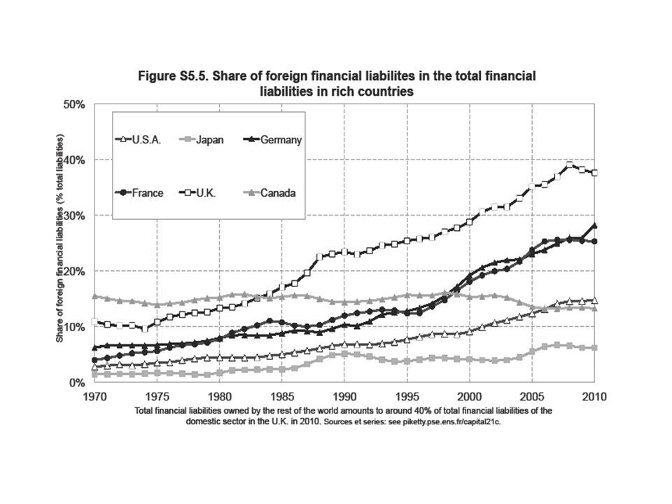
61. Gross vs net foreign assets: financial globalization in action Net foreign asset positions are smaller today than what they were in 1900-1910 But they are rising fast in Germany, Japan and oil countries And gross foreign assets and liabilities are a lot larger than they have ever been, especially in small countries: about 30-40% of total financial assets and liabilities in European countries (even more in smaller countries) This potentially creates substantial financial fragility (especially if link between private risk and sovereign risk) This destabilizing force is probably even more important than the rise of top income shares (=important in the US, but not so much in Europe; see lecture 5 & PS, « Top incomes and the Great Recession », IMF Review 2013 )IMF Review 2013

72. Market vs book value of corporations So far we used a market-value definition of national wealth W n : corporations valued at stock market prices Book value of corporations = assets – debt Tobin’s Q ratio = (market value)/(book value) (>1 or <1) Residual corporate wealth W c = book value – market value Book-value national wealth W b = W n + W c In principe, Q ≈ 1 (otherwise, investment should adjust), so that W c ≈ 0 and W b ≈ W n But Q can be systematically >1 if immaterial investment not well accounted in book assets But Q can be systemativally <1 if shareholders have imperfect control of the firm (stakeholder model): this can explain why Q lower in Germany than in US-UK, and the general rise of Q since 1970s-80s From an efficiency viewpoint, unclear which model is best

74. Summing up Wealth-income ratios β and β n have no reason to be stable over time and across countries If global growth slowdown in the future (g≈1,5%) and saving rates remain high (s≈10-12%), then the global β might rise towards 700% (or more… or less…) Major issue: can depreciation of natural capital be stronger than the rise of private capital? See Barbier 2014a, 2014b Barbier 2014a2014b What are the consequences for the share α of capital income in national income? See next lecture

76. Capital-income ratios β vs. capital shares α Capital/income ratio β=K/Y Capital share α = Y K /Y with Y K = capital income (=sum of rent, dividends, interest, profits, etc.: i.e. all incomes going to the owners of capital, independently of any labor input) I.e. β = ratio between capital stock and income flow While α = share of capital income in total income flow By definition: α = r x β With r = Y K /K = average real rate of return to capital If β=600% and r=5%, then α = 30% = typical values

77. In practice, the average rate of return to capital r (typically r≈4-5%) varies a lot across assets and over individuals (more on this in Lecture 6) Typically, rental return on housing = 3-4% (i.e. the rental value of an appartment worth 100 000€ is generally about 3000-4000€/year) (+ capital gain or loss) Return on stock market (dividend + k gain) = as much as 6-7% in the long run Return on bank accounts or cash = as little as 1-2% (but only a small fraction of total wealth) Average return across all assets and individuals ≈ 4-5%

78. The Cobb-Douglas production function Cobb-Douglas production function: Y = F(K,L) = K α L 1-α With perfect competition, wage rate v = marginal product of labor, rate of return r = marginal product of capital: r = F K = α K α-1 L 1-α and v = F L = (1-α) K α L -α Therefore capital income Y K = r K = α Y & labor income Y L = v L = (1-α) Y I.e. capital & labor shares are entirely set by technology (say, α=30%, 1-α=70%) and do not depend on quantities K, L Intuition: Cobb-Douglas ↔ elasticity of substitution between K & L is exactly equal to 1 I.e. if v/r rises by 1%, K/L=α/(1-α) v/r also rises by 1%. So the quantity response exactly offsets the change in prices: if wages ↑by 1%, then firms use 1% less labor, so that labor share in total output remains the same as before

79. The limits of Cobb-Douglas Economists like Cobb-Douglas production function, because stable capital shares are approximately stable However it is only an approximation: in practice, capital shares α vary in the 20-40% range over time and between countries (or even sometime in the 10-50% range) In 19c, capital shares were closer to 40%; in 20c, they were closer to 20-30%; structural rise of human capital (i.e. exponent α↓ in Cobb-Douglas production function Y = K α L 1-α ?), or purely temporary phenomenon ? Over 1970-2010 period, capital shares have increased from 15- 25% to 25-30% in rich countries : very difficult to explain with Cobb-Douglas framework

83. The CES production function CES = a simple way to think about changing capital shares CES : Y = F(K,L) = [a K ( σ-1)/σ + b L ( σ-1)/σ ] σ/(σ-1) with a, b = constant σ = constant elasticity of substitution between K and L σ →∞: linear production function Y = r K + v L (infinite substitution: machines can replace workers and vice versa, so that the returns to capital and labor do not fall at all when the quantity of capital or labor rise) ( = robot economy) σ →0: F(K,L)=min(rK,vL) (fixed coefficients) = no substitution possibility: one needs exactly one machine per worker σ →1: converges toward Cobb-Douglas; but all intermediate cases are also possible: Cobb-Douglas is just one possibility among many Compute the first derivative r = F K : the marginal product to capital is given by r = F K = a β -1/ σ (with β=K/Y) I.e. r ↓ as β↑ (more capital makes capital less useful), but the important point is that the speed at which r ↓ depends on σ

84. With r = F K = a β -1/ σ, the capital share α is given by: α = r β = a β ( σ -1)/ σ I.e. α is an increasing function of β if and only if σ>1 (and stable iff σ=1) The important point is that with large changes in the volume of capital β, small departures from σ=1 are enough to explain large changes in α If σ = 1.5, capital share rises from α=28% to α =36% when β rises from β=250% to β =500% = more or less what happened since the 1970s In case β reaches β =800%, α would reach α =42% In case σ =1.8, α would be as large as α =53%

88. Measurement problems with capital shares In many ways, β is easier to measure than α In principle, capital income = all income flows going to capital owners (independanty of any labor input); labor income = all income flows going to labor earners (independantly of any capital input) But in practice, the line is often hard to draw: family firms, self- semployed workers, informal financial intermediation costs (=the time spent to manage one’s own portfolio) If one measures the capital share α from national accounts (rent+dividend+interest+profits) and compute average return r=α/β, then the implied r often looks very high for a pure return to capital ownership: it probably includes a non-negligible entrepreneurial labor component, particularly in reconstruction periods with low β and high r; the pure return might be 20-30% smaller (see estimates) Maybe one should use two-sector models Y=Y h +Y b (housing + business); return to housing = closer to pure return to capital

96. Recent work on capital shares Imperfect competition and globalization: see Karabarmounis-Neiman 2013, « The Global Decline in the Labor Share »; see also KN2014 Karabarmounis-Neiman 2013KN2014 Atkinson-Summers: Y=F(K 1,AL+BK 2 ) Public vs private firms: see Azmat-Manning-Van Reenen 2011, « Privatization and the Decline of the Labor Share in GDP: A Cross-Country Aanalysis of the Network Industries »Azmat-Manning-Van Reenen 2011 Capital shares and CEO pay: see Pursey 2013, « CEO Pay and Factor shares: Bargaining effects in US corporations 1970-2011 »Pursey 2013

97. Summing up The rate of return to capital r is determined mostly by technology: r = F K = marginal product to capital, elasticity of substitution σ The quantity of capital β is determined by saving attitudes and by growth (=fertility + innovation): β = s/g The capital share is determined by the product of the two: α = r x β Anything can happen

98. Note: the return to capital r=F K is dermined not only by technology but also by psychology, i.e. saving attitudes s=s(r) might vary with the rate of return In models with wealth or bequest in the utility function U(c t,w t+1 ), there is zero saving elasticity with U(c,w)=c 1-s w s, but with more general functional forms on can get any elasticity In pure lifecycle model, the saving rate s is primarily determined by demographic structure (more time in retirement → higher s), but it can also vary with the rate of return, in particular if the rate of return becomes very low (say, below 2%) or very high (say, above 6%)

99. In the dynastic utility model, the rate of return is entirely set by the rate of time preference (=psychological parameter) and the growth rate: Max Σ U(c t )/(1+δ) t, with U(c)=c 1-1/ξ /(1-1/ξ) → unique long rate rate of return r t → r = δ +ξg > g (ξ>1 and transverality condition) This holds both in the representative agent version of model and in the heteogenous agent version (with insurable shocks); more on this in Lecture 6