1. Extratropical Air-Sea Interaction and Patterns of Climate Variability Michael Alexander NOAA/Earth System Research Lab Physical Science Division

2. Overview Processes that influence upper ocean temperature and mixed layer depth Patterns of variability –Atmospheric e.g NAO –and their impact on the ocean NAO => SST tripole Process that impact ocean patterns –Nonlinear interactions & weather forcing of the ocean –Ocean Mixed layer dynamics: “Reemergence Mechanism” –ENSO teleconnections: “Atmospheric Bridge” –Changes in ocean gyres –MOC/THC (Delworth)

3. SST Tendency Equation Variables v - velocity (current in ML) (vek, vg) T m – mixed layer temp (SST) T b – temp just beneath ML h – mixed layer depth w – mean vertical velocity w e – entrainment velocity Q net – net surface heat flux Q swh – penetrating shortwave radiation A –horizontal eddy viscosity coefficient e.g. see Frankignoul (1985, Rev. Geophysics) Integrated heat budget over the mixed layer:

4. Extratropical Patterns of Variability Weather Maps - dominated by moving storms On weekly and longer time scales larger stationary atmospheric patterns emerge These patterns are mainly due to internal atmospheric variability (e.g. interactions with storm tracks, flow over mountains, etc). but can also be influenced by the ocean, sea ice, global warming, etc. The atmospheric patterns strongly influence the underlying ocean

5. NH Teleconnection Patterns in upper atm NAO/AO/ NAM TNH NPO/WP PNA

6. North Atlantic Oscillation (NAO) Deser et al. 2009

7. NPO=> North Pacific Gyre Oscillation (NPGO) Di Lorenzo et al 2007, 2009

8. Southern Annular Mode (SAM) Nov-MarMay-Oct Ciasto and Thompson, 2008, J. Climate

9. What are the underlying characteristics of atmospheric variability? How do these patterns evolve with time?

10. Linear, Nonlinear Interactions and Chaotic systems Linear: y = ax, a is constant, x is variable e.g. dT/dt = U dT/dx; U mean wind Time Nonlinear: y = zx; z variable e.g dT/dx = u dT/dx; u actual wind T

11. Nonlinear Interactions Impact on Climate Asymmetry: e.g El Niño different than La Niña For atmosphere, coupled models or eddy resolving ocean models,need an ensemble of simulations to isolate a forced signal A given year of a “20th century” simulation (with all observed forcings will not match the corresponding year in nature There is only very limited predictability (perhaps due to coupled air-sea interaction) of patterns like the NAO beyond a few weeks For air-sea interaction can consider nonlinear terms as “weather noise” and the ocean response as a slower and linear => “stochastic model”

12. Southern Annular Mode SLP (65º-71ºS minus 37º-47ºS) Linear Trend 2000-2061 Coupled Model (CCSM3) with A1B GHG forcing Dots: Individual Ensemble Members Line: 40-member Ensemble Mean stronger weaker westerlies Member 11Member 13 0 hPa / 62yrs 5 -5 Nov-Mar

13. Simple model for generating SST variability “stochastic model” Heat fluxes associated with weather events, “random forcing” Ocean response to flux back heat which slowly damps SST anomalies SST anomalies form Air-sea interface Fixed depth ocean No currents Bottom d(SST´)/dt = F´ -  SST´)  ch

14. Stochastic Model Example: flux forcing and SST times series SST n+1 = *SST n +  =constant;  = Random number

15. Seasonal cycle of Temperature & MLD in N. Pacific Reemergence Mechanism Winter Surface flux anomalies Create SST anomalies which spread over ML ML reforms close to surface in spring Summer SST anomalies strongly damped by air-sea interaction Temperature anomalies persist in summer thermocline Re-entrained into the ML in the following fall and winter Q net ’ Alexander and Deser (1995, JPO), Alexander et al. (1999, J. Climate) MLD

16. Reemergence in three North Pacific regions Regression between SST anomalies in April-May with monthly temperature anomalies as a function of depth. Regions Alexander et al. (1999, J. Climate)

17. Watanabe and Kimoto (2000); Timlin et al. 2002, Deser et al 2003 (J.Clim), De Coetlogon and Frankignoul 2003 : all J. Climate Auto-correlation of EOF PC time series Level of significance Degrees Celsius Reemergence of the SST North Atlantic tripole Leading EOF of March SST ERSSTv2 Datasets [1950-2003] Reemergence of SST Tripole

18. “The Atmospheric Bridge” Meridional cross section through the central Pacific (Alexander 1992; Lau and Nath 1996; Alexander et al. 2002 all J. Climate)

19. Global ENSO Signal (SST shaded, SLP contour, ci = 1mb)

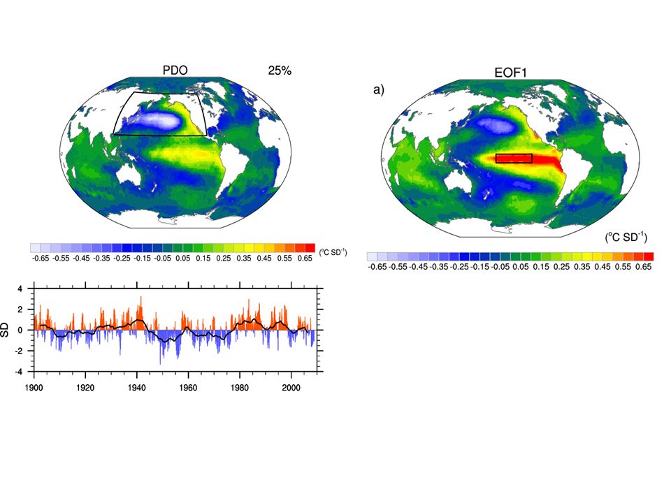
20. Leading Pattern (1st EOF) of North Pacific SST + Phase - Phase K Mantua et al. (BAMS 1997) PC 1 SST North Pacific The Pacific Decadal Oscillation (PDO) H

21. What Causes Midlatitude Anomalies SSTs? The PDO? and Pacific Decadal Variability in General? Random forcing by the Atmosphere –Aleutian low => underlying ocean Signal from the Tropics? –Midlatitudes integrates ENSO interannual signal –decadal variability in the ENSO region Midlatitude Dynamics –Shifts in the strength/position of the ocean gyres –Could include feedbacks with the atmosphere

22. Aleutian Low Impact on Fluxes & SSTs in (DJF) Leading Patterns of Variability AGCM-MLM EOF 1 SLP (50%) SLP PC1 - Qnet correlation SLP PC1 - SST correlation EOF 1 SST (34%)

23. PDO or slab ocean forced by noise? Pierce 2001, Progress in Oceanography

24. SLP & SST Patterns of Pacific Variability ENSOPDO Regressions: SLP – Contour; SST Shaded Mantua et al. 1997, BAMS

25. El Niño – La Niña Composite: Model Obs DJF SLP Contour (1 mb); FMA SST (shaded ºC) reemergence

26. Pacific Ocean Currents Annual average ocean currents (m s -1 ) averaged over the upper 500 m from the Simple Ocean Data Assimilation (SODA, Carton and Giese, 2008) for the years 1958-2001. The current strength is indicated by the three tone gray scale with maximum values of ~0.7 m sec -1 in the Kuroshio. Subtropical gyre Subpolar gyre

27. Wind Generated Rossby Waves West East Atmosphere Ocean Thermocline ML L Rossby Waves 1)After waves pass ocean currents adjust 2)Waves change thermocline depth, if mixed layer reaches that depth, cold water can be mixed to the surface

28. Rossby wave propagation Qiu et al. 2007

29. SST anomalies and spectra in KE region Stochastic model

30. Ocean Response to Change in Wind Stress Contours: geostrophic flow from change in wind stress Shading: vertically integrated temperature (0-450 m): 1982-90 – 1970-80 Deser, Alexander & Timlin 1999 J. Climate SLP 1977-88 - 1968-76

31. PDO Reconstruction 41% 38% 7% 85% >8years 75% 20% 31% 24% Schneider and Cornuelle 2005 J Climate Forcings (F) ENSO Aleutian Low ∆ in Gyres

32. Prediction of the PDO Monthly values PDO Index 1998 Transition? Curve Extrapolation Because of the multiple contributions to the PDO some of which are due to unpredictable atmospheric fluctuations PDO predictable out to 1-2 year Unclear if “regimes”, jumping between two different states (implies low order chaos). More likely impact of multiple processes that can add together to get rapid changes

33. Hare and Mantua, 2000 Alaska Sockeye Salmon Catch Western Central Southeast 19761988 1995198519751965

34. Summary Climate noise –Expect decadal variability when looking at SST time series Atmospheric Bridge –Cause and effect well understood –Tropical Pacific => Global SSTs –Influence of air-sea feedback on extratropical atmosphere complex PDO (1 st EOF of North Pacific SST) –Thermal response to random fluctuations in Aleutian Low –A significant fraction of the signal comes from the tropics Extratropical ocean integrates (reddens) ENSO signal Decadal variability in tropics – impact atmosphere & ocean –extratropical air-sea feedback modest amplitude (1/4 -1/3 of ENSO signal) Other Processes/modes of variability –Ocean currents & Rossby waves in N. Pacific and N. Atlantic –Changes in the Thermohaline Circulation =?=> AMO, AMM

35. El Niño– La Niña composite average a) surface wind stress vectors (N m -2, and SST (b) net surface heat flux c) Ekman transport in flux form during JF(1) as obtained from NCEP reanalysis for ENSO events during the period 1950-1999. L represents the center of the anomalous negative SLP anomaly associated with a deeper Aleutian low and the red (blue) arrows indicate the direction of Ekman transport that warms (cools) the ocean. Observed Atmos. Bridge Fluxes

36. Midlatitude SST Variability The ocean primarily influences the atmosphere through changes in the SST There are many ways that SST anomalies form –We will explore just a few mechanisms –Ones that are part of larger climate signals Mechanisms for generating midlatitude SST anomalies –Climate Noise Random forcing of the ocean –Upper Ocean mixing processes –“Atmospheric Bridge”: Teleconnections with ENSO –Changes in ocean currents Wind driven (through ocean Rossby waves) Thermal/salt driven: Thermohaline

37. Observed Standard Deviation of SST Anomalies (°C) August March

38. Additional Slides More on the experiment of reemergence in the Atlantic Rossby waves that are

39. Simple Ocean Model: correspondence to the real world? Observed and Theoretical Spectra for a location in the North Atlantic Ocean Theoretical spectra of Simple ocean model Observed OWS Temperature Variance 1 year1 month (Hz) is the frequency period: Atmospheric forcing and ocean feedback estimated from data

40. The Simple Ocean’s SST Anomaly Variability Log plot of SSTA Spectra Period 1yr 10 yr No damping SSTA Variance 1 mo Atm forcing Frequency (  ) SST(  ) 2 = |F| 2  2 + 2

42. Wet Precipitation (land only) Dry 180° Warm Cold Surface Air Temperature 180° Precipitation and Temperature Patterns Associated with NP (and PDO) Index

43. Ocean Mixed layer Turbulence creates a well mixed surface layer where temperature (T), salinity (S) and density (  ) are nearly uniform with depth Primarily driven by vertical processes (assumed here) but can interact with 3-D circulation Density jump usually controlled by temperature but sometimes by salinity (especially in high latitudes) Often “ measured” by the depth at which T is some value less than SST (e.g. ∆T = 0.5) Under goes large seasonal cycle This impacts the evolution of ocean temperature anomalies and has important biological consequences  T s  ∆T

44. Seasonal Cycle of Temp & MLD the Northeast Pacific (50ºN, 145ºW)

45. Climatological Mixed Layer Depth (m)

46. Do the reemerging SST anomalies impact the atmosphere? First examine relationship between atmospheric circulation and SSTs in the Atlantic to determine leading pattern of SSTs forced in winter and see if they reemerge Then use AGCM (NCAR CAM2) coupled to a mixed layer ocean model (predicts h) Cassou, Deser and Alexander (J Climate 2007)

47. March SST EOF1 (shade) Regressed JFM SLP (contour) PC time series: March SST (bars), JFM MSLP (line) NCEP MSLP [1950-2003] Correlation=0.63 e.g. Deser and Timlin (1997), J.Clim. Atmosphere forcing the ocean in winter: NAO & the Atlantic SST tripole

48. Summary Entainment & concept of MLD important for SST evolution –E.g. SST anomalies larger in summer than winter due to shallow MLD Reemergence –Adds predictability for SST and potentially for the atmosphere as well –Extends the stocashtic model for SSTs –Also occurs for salinity –Reemergence extends oceanic impact of atmospheric teleconnections Other roles for mixing –Interaction with the deeper ocean Subduction (ML water leaves the surface) Rossby wave propagation to the Kuroshio region: –Remix temperature anomalies due to thermocline variability back to the surface –Biological Bring nutrients to the surface (if not enough nutrient limited) Mix phytoplankton if too much (light limited)

49. Nov-FebJul-OctMar-Jun 40-member CCSM3 10,000 year atmospheric model (CAM3) control integration Standard Deviation of SLP Trends Lack of stippling indicates standard deviations are not significantly different between CCSM3 and CAM3 control integration (i.e., spread in CCSM3 trends is consistent with internal atmospheric variability or “weather noise”)

50. 1. What is the oceanic reemergence? 2. Surface signature of reemergence in the Labrador Sea Sea Surface Temperature e-folding = ~ 4 mths Auto-correlation of the Labrador SST time series (all months considered), e.g. for lag=1, Jan50/Feb50/…/Dec00 values are correlated with Feb50/Mar50/…/Jan01 values e-folding = ~ 36 mths e-folding = ~ 4 mths Auto-correlation of the Labrador SST time series (Starting from March), e.g. for lag=1, March and April time series are correlated, for lag =2 March and May etc. Reemergence of the late winter SST anomalies a year after Deser et al. 2003 (J.Clim) ERSSTv2 Datasets [1950-2003] Degrees Celcius Level of significance

51. Atmosphere-Ocean Ice Model Atmospheric GCM – NCAR CAM2–T42 resolution Ice Thermodynamic portion of NCAR CSIMv4 Ocean Mixed layer Model (MLM) An individual column model with a uniform mixed layer Atop a layered model that represents conditions in the pycnocline Prognostic ML depth Same grids as the atmosphere (128 lon x 64 lat) 36 vertical levels (from 0m to 1500m depth) higher resolution close to surface and a realistic bathymetry Flux correction needed to get reasonable climate Cassou et al. 2007 J Clim; Alexander et al. 2000 JGR, Alexander et al 2002 – J.Clim ; Gaspar 1988 – JPO

52. Additional Topics The flux components and their variability Schematic of the mixed layer model Pattern of atmospheric circulation (SLP) and the underlying fluxes) Basin-wide reemergence The Pacific Decadal Oscillation Wind generated Rossby waves and its relation to SSTs The Latif and Barnett mechanism for the PDO and “problems” with this mechanism

53. Observed Rossby Waves & SST Schneider and Miller 2001 (J. Climate) March KE Region: 40°N, 140°-170°E SST OB S T 400 SST fcst Correlation Obs SST hindcast With thermocline depth anomaly Forecast equation for SST based on integrating wind stress (curl) forcing and constant propagation speed of the (1 st Baroclinic) Rossby wave

54. Forecast Skill: Correlation with Obs SST Wave Model & Reemergence Wave ModelReemergence years Schneider and Miller 2001 (J. Climate)

55. Evolution of the leading pattern of SST variability as indicated by extended EOF analyses Alexander et al. 2001, Prog. Ocean. No ENSO; Reemergence ENSO; No Reemergence

56. Mechanism for Atmospheric Circulation Changes due to El Nino/Southern Oscillation Horel and Wallace, Mon. Wea Rev. 1981 Latent heat release in thunderstorms Atmospheric wave forced by tropical heating

57. Conclusions The Atlantic Meridional Mode (AMM) is strongly related to Atlantic hurricane activity »The AMM is associated with a set of large-scale conditions that all cooperate in their influence on hurricane activity »The AMM increases seasonal intensity because: There are more storms They track through climatologically, and anomalously, favorable environmental conditions Their duration is increased, allowing more time to intensify The AMM is predictable up to a year in advance.

58. Conclusions The AMM provides a better framework for understanding existing hurricane / climate relationships in the Atlantic »The AMM represents an organizing “mode” of climate variability in the tropical Atlantic »The strong relationship between SST and the AMM suggests that SST is strongly related to hurricane activity because it is a good proxy for the AMM »The AMM is related not only to intensity, but also to frequency and duration. As such, its influence on seasonal hurricane intensity metrics is larger than would be predicted by simple thermodynamic arguments

59. PDO: Multiple Causes Newman, Compo, Alexander 2003, Schneider and Miller 2005, Newman 2006 (All in Journal of Climate) Interannual timescales: –Integration of noise (Fluctuations of the Aleutian Low) –Response to ENSO (Atmospheric bridge) –+ Reemergence Decadal timescales (% of Variance) –Integration of noise (1/3) –Response to ENSO (1/3) –Ocean dynamics (1/3) –Predictable out to (but not beyond) 1-2 years Trend –Most Prominent in Indian Ocean and far western Pacific –A portion associated with Global warming