Download presentation
Presentation is loading. Please wait.

1
Lecture I: The Time-dependent Schrodinger Equation A. Mathematical and Physical Introduction B. Four methods of solution 1. Separation of variables 2. Parametrized functional form 3. Method of characteristics 4. Numerical methods

2
H is a Hermitian operator is a complex wavefunction Normalization has physical interpretation as a probability density A is an anti-Hermitian operator on a complex Hilbert space Inner product on a complex Hilbert space Math Perspective: Complex wave equation Physics Perspective: Time-dependent Schrodinger eq.

3
Integral representation for Proof of norm conservation Math Perspective: Complex wave equation Physics Perspective: Time-dependent Schrodinger eq.

4
Solution of the time-dependent Schrodinger equation Method 1: Separation of variables Ansatz: Time-independent Schrodinger eq has solutions that satisfy boundary conditions in general only for particular values of

5
Solutions of the time-independent Schrodinger equation particle in a box (discrete) harmonic oscillator (discrete) Morse oscillator (discrete +continuous) IV Eckart barrier (degenerate continous )
 harmonic oscillator (discrete) Morse oscillator (discrete +continuous) IV Eckart barrier (degenerate continous )")
6
Reconstituting the wavefunction (x,t)
")
7
Example: Particle in half a box

9
Solution of the time-dependent Schrodinger equation Method 2: Parametrized functional form For the ansatz: leads to the diff eqs for the parameters:

10
Solution of the time-dependent Schrodinger equation Method 2: Parametrized functional form For the ansatz: leads to the diff eqs for the parameters: Hamilton’s equations (classical mechanics) Classical Lagrangian (Ricatti equattion)
 Classical Lagrangian (Ricatti equattion)")
12
Squeezed state Coherent state Anti-squeezed state

13
Ehrenfest’s theorem and wavepacket revivals Ehrenfest’s theorem Wavepacket revivals On intermediate time scales for anharmonic potentials Ehrenfest’s theorem quite generally breaks down. However, on still longer time scales there is, in many cases of interest, an almost complete revival of the wavepacket and a second Ehrenfest epoch. In between these full revivals are an infinite number of fractional revivals that collectively have an interesting mathematical structure.

14
Ehrenfest’s theorem and wavepacket revivals Ehrenfest’s theorem Wavepacket revivals

15
Wigner phase space representation

16
Harmonic oscillator Coherent state Squeezed stateAnti-squeezed state

17
Wigner phase space representation Particle in half a box

18
Solution of the time-dependent Schrodinger equation Method 3: Method of characteristics Ansatz: LHS is the classical HJ equation: phase action RHS is the quantum potential: contains all quantum non-locality continuity equation quantum HJ equation

19
From the quantum HJ equation to quantum trajectories Quantum force-- nonlocal total derivative=“go with the flow” Classical HJ equation Classical trajectories Quantum HJ equation Quantum trajectories

20
Reconciling Bohm and Ehrenfest The LHS is the classical Hamilton-Jacobi equation for complex S, therefore complex x and p (complex trajectories). The RHS is the quantum potential which is now complex. Complex quantum Hamilton-Jacobi equation ! Complex S ! Complex quantum potential

21
Reconciling Bohm and Ehrenfest For Gaussian wavepackets in potentials up to quadratic, the quantum force vanishes! Complex quantum Hamilton-Jacobi equation ! Complex S ! Complex quantum potential

22
Solution of the time-dependent Schrodinger equation Method 4: Numerical methods Digression on the momentum representation and Dirac notation

23
Solution of the time-dependent Schrodinger equation Method 4: Numerical methods Digression on the momentum representation and Dirac notation

24
Solution of the time-dependent Schrodinger equation Method 4: Numerical methods

25
Increase accuracy by subdividing time interval:

26
From the the split operator to classical mechanics: Feynman path integration evolution operator or propagator titi t i+1 0 t x’x

27
From the the split operator to classical mechanics: Feynman path integration evolution operator or propagator titi t i+1 0 t x’x

28
From the the split operator to classical mechanics: Feynman path integration

30
Lecture II: Concepts for Chemical Simulations A. Wavepacket time-correlation functions 1. Bound potentials Spectroscopy 2. Unbound potentials Chemical reactions B. Eigenstates as superpositions of wavepackets C. Manipulating wavepacket motion 1. Franck-Condon principle 2. Control of photochemical reactions

31
A.Wavepacket correlation functions for bound potentials

32
Particle in half a box

33
A. Wavepacket correlation functions for bound potentials Harmonic oscillator

34
A. Wavepacket correlation functions for bound potentials

35
A. Wavepacket correlation functions for unbound potentials Eckart barrier Correlation function and spectrum of incident wavepacket

36
Correlation function and spectrum of reflected and transmitted wavepackets

37
Normalizing the spectrum to obtain reflection and transmission coefficients

38
B. Eigenfunctions as superpositions of wavepackets eigenfunction wavepacketsuperposition

39
B. Eigenfunctions as superpositions of wavepackets eigenfunction wavepacket superposition

40
B. Eigenfunctions as superpositions of wavepackets eigenfunction wavepacket superposition n=1 E=1.5 2<n<3 E=3.0 n=7 E=7.5

41
B. Eigenfunctions as superpositions of wavepackets eigenfunction wavepacket superposition

42
C. Manipulating Wavepacket Motion Franck-Condon principle

43
C. Manipulating Wavepacket Motion Franck-Condon principle

44
C. Manipulating Wavepacket Motion Franck-Condon principle—a second time

45
C. Manipulating Wavepacket Motion 1. Franck-Condon principle photodissociation

46
C. Manipulating Wavepacket Motion Control of photochemical reactions Laser selective chemistry: Is it possible? dissociation isomerization ring opening C H O H CC H H H H C H C CC H O H

47
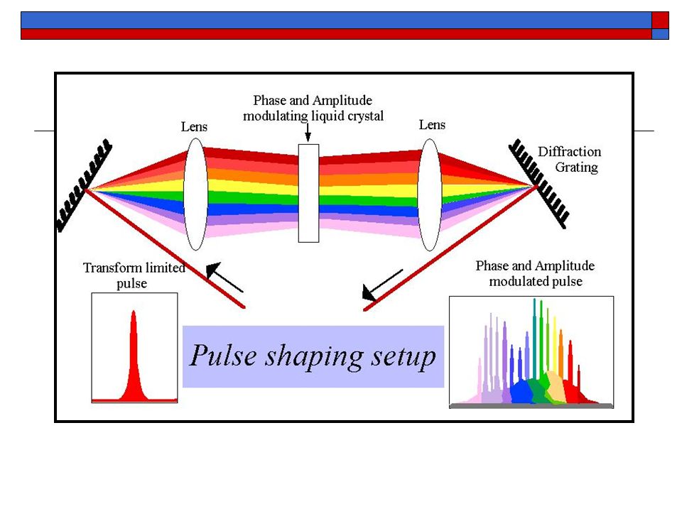
Wavepacket Dancing: Chemical Selectivity by Shaping Light Pulses 1. Review of Tannor-Rice scheme 2. Calculus of Variations Approach 3. Iterative Approach and Learning Algorithms (Tannor, Kosloff and Rice, 1985, 1986)
.")
49
Tannor, Kosloff and Rice (1986)
")
51
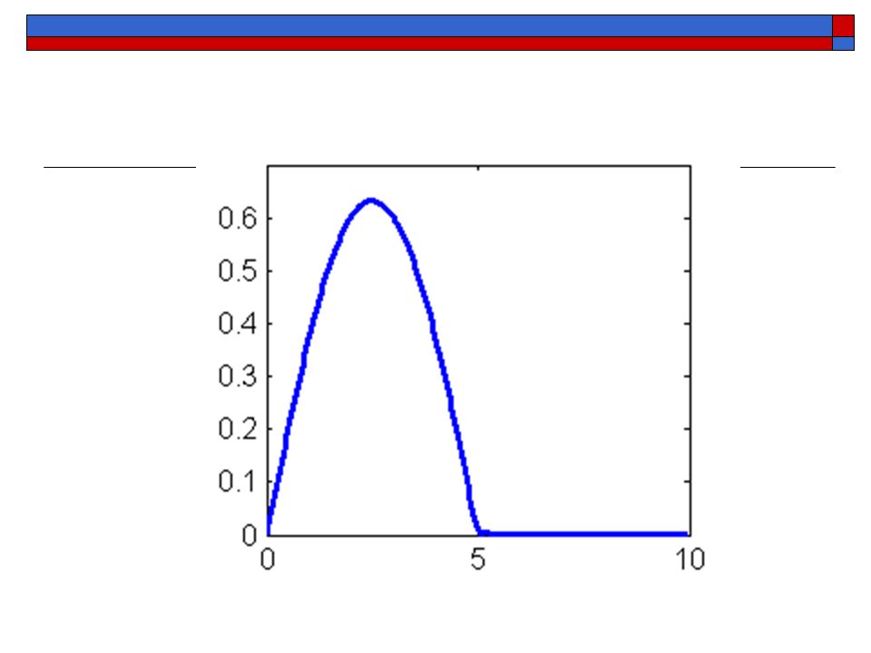
Optimal Pulse Shapes

52
J is a functional of : calculus of variations

53
Formal Mathematical Approach A. Calculus of Variations (technique for finding the “best shape” (Tannor and Rice, 1985) 1. Objective functional P is a projection operator for chemical channel 2. Constraint (or penalty) B. Optimal Control (Peirce, Dahleh and Rabitz, 1988) (Kosloff,Rice,Gaspard,Tersigni and Tannor (1989) 3. Equations of motion are added to “deconstrain” the variables
 1. Objective functional P is a projection operator for chemical channel 2. Constraint (or penalty) B. Optimal Control (Peirce, Dahleh and Rabitz, 1988) (Kosloff,Rice,Gaspard,Tersigni and Tannor (1989) 3. Equations of motion are added to deconstrain the variables.")
54
Modified Objective Functional

55
(i)(ii)(iii)
(ii)(iii)")
56
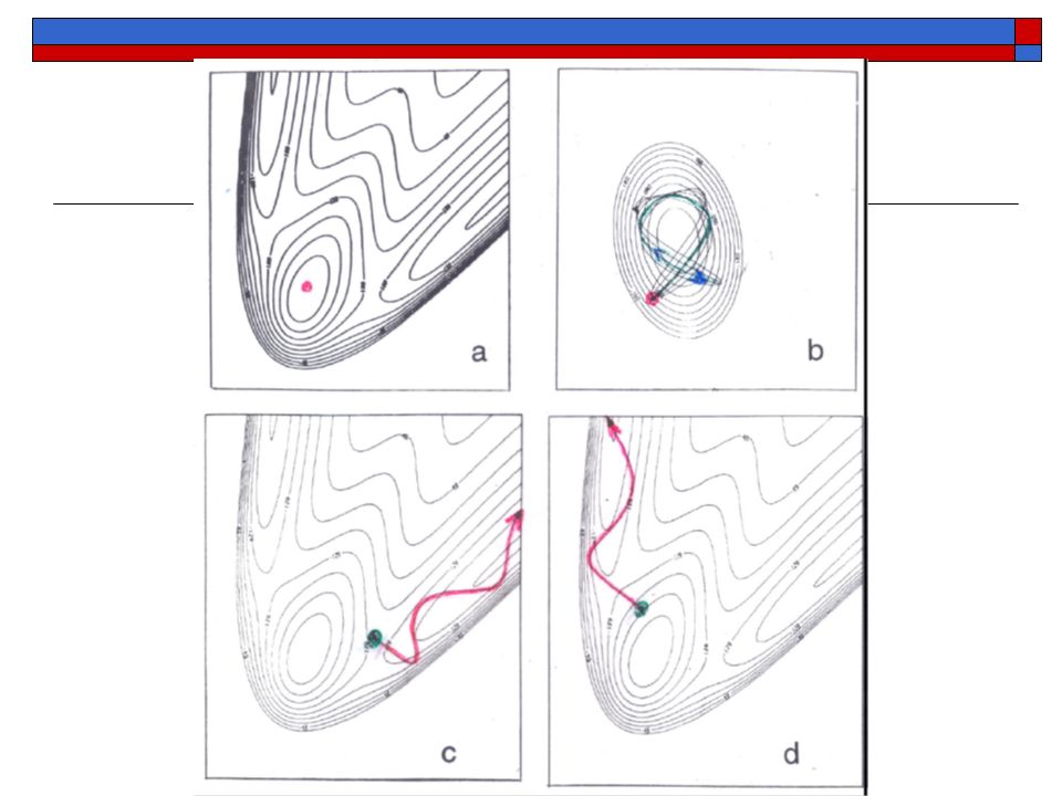
equations of motion for equations of motion for optimal field equations of motion for Iterate! Tannor, Kosloff, Rice (1985-89) Rabitz et al. (1988) Optimal Control: Iterative Solution
 Rabitz et al. (1988) Optimal Control: Iterative Solution.")
Similar presentations


>")


, Ch.6.1-3: Schrödinger.>")

 - operators (representing observables)>")
