1. 501 PHYS
ِProf. Awatif Ahmad Hindi
ُEnter

2. Reference
1- W.E boyce and R.C Diprema , "elementary differential equations " 3rd edition (1975), johnwily
2- E.A coddington , “ an introduction to ordinary differential equation “ , prentice –hali (1961)
3- E.Kreyszig “advanced engineering mathematics “ 7th edition , johnwily (1993)
4- L.S. ross , “introduction to ordinary differential equations” 4th edition , john wily (1989)
5- Abramowitz , M. stegun , I.A. hand book of mathematical function . dover, new York (1962)

3. Reference
6- hochstadt , H. “special function of mathematical physics “ hold , rineheart , winstone , new york (1961)
7- Lebedev,N.N.Special Functions and their Applications,Prentice-Hall,Englewood Cliffs,N.J.(1965)
8-Rainvile,E.D.”Special Functions,Macmillan,New York(1960).

4. contents Special Functions of mathematics Integral Equation
Differential equation

5. Special Functions of mathematics Gamma and Beta functions
Definition
Properties of the Beta and Gamma functions:
some examples

6. Definition
We define the Gamma and Beta functions respectively by

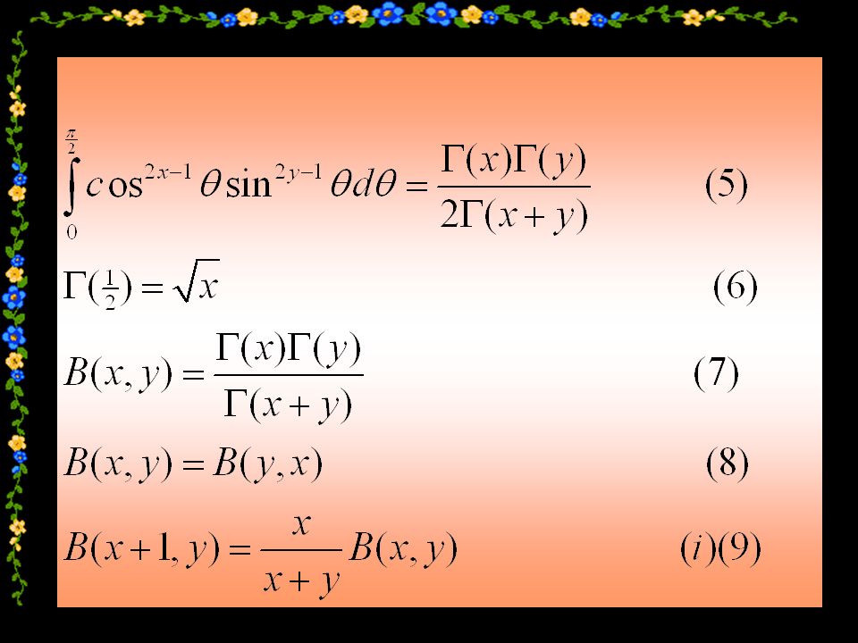
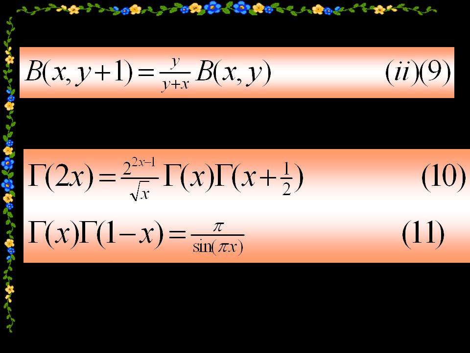
7. Properties of the Beta and Gamma
functions:

10. Definition of the Gamma function for negative values of the argument

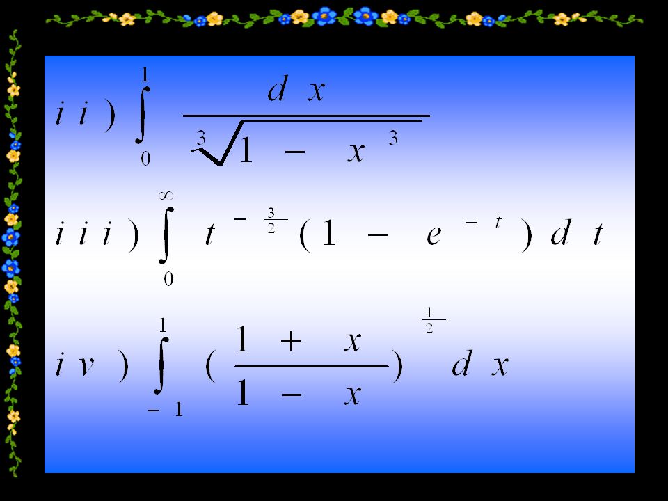
11. simplify where possible
Some examples
Express each of the following integrals in terms of Gamma or Beta functions and
simplify where possible

13. Bessel Functions Bessel’s equation of order n is
We shall solve (1)by using Frobinous method the solution of (1) is given by :

14. The explicit relation ship between
and
for integral n is
shown in the following theorems
Theorem 4
Theorem 1
Theorem 5
Theorem 2
Theorem 6
Theorem 3
Theorem 7

15. Theorem 1
When n is an integer (positive or negative)

16. The two independent solutions of Bessel’s equation may be taken to be
Theorem 2
The two independent solutions of Bessel’s equation may be taken to be
For all values of n.

17. Generating function for the Bessel functions
Theorem 3
Generating function for the Bessel functions

18. Integral representations for Bessel functions:
Theorem 4
Integral representations for Bessel functions:

19. Theorem 5

20. Recurrence Relations

21. graphs of the Bessel functions

22. graphs of the Bessel functions

23. graphs of the Bessel functions

24. Orthogonally of the Bessel functions
Theorem 6
Orthogonally of the Bessel functions If
are roots of the equation

25. Theorem 7 Bessel Series If f(x) is defined in the region
and can be expanded in the form
Where the
are the roots of the equation
then

26. problems
1-Use the generating function to prove that
2- Show that

27. Integral equation
Definition(1)
Defintion (2)
Defintion (3)

28. Integral equation Definition(1)) An integral equation is an equation
in which an unknown function
appears under one or more integral signs.
Naturally, in such an equation there
can occur other terms as well .

29. For example
The equation
for
for

30. Where the function is the unknown function which all the
functions are known are integral equation .
These functions may be complex –valued functions
of the variables S and t
for

31. Integral equation Definition(2))
An integral equation is called linear if only linear
operations are performed function on it upon the
unknown function .
The equations (1) and (2) are Linear while (3) is nonlinear.

32. Integral equation Definition(3))
The most general type of linear integral equation is of the form:
Where the upper limit be either variable or fixed.
The functions are known functions,

33. While is to be determined ; is a nonzero,real or complex, parameter
for
is called the kernel .
Is called the Kernel

34. The following special cases of equation (4) are of main interest :
I) Fredholm integral equation
II) Volterra Equations

35. I) Fredholm integral equation:
In all Fredholm integral equation of the first kind the upper limit of integration b,say,is fixed.
i) In the Fredholm integral equation of the first kind Thus,
= (5)

36. I) Fredholm integral equation:
ii) In the Fredholm integral equation of the second
kind,

37. I) Fredholm integral equation:
iii) The homogeneous Fredholm integral equation
of the second kind is a special case of(ii) above .
In this case

38. II) Volterra Equations
Volterra Equations of the first, homogeneous ,
and second kinds are precisely as above except that
is the variable upper limit of integration.
Equation (4) itself is called an integral equation of
the third kind

39. Singular Integral equation:
Definition (4)
When one or both limits of integration become
infinite or when the kernel becomes infinite at
one or more points within the range of
integration ,the integral equation is
called Singular .

40. Are singular integral equations.
For example ,the Integral equations
Are singular integral equations.

41. Special Kinds of kernel
separable or degenerate kernels
Symmetric kernel

42. I) separable or degenerate kernels
A kernel to k(s,t) is called separable or
degenerate if it can be expressed as the
sum of a finite number of terms each of
which is the product of a function s only
and a function of only
; that is,

43. II) Symmetric kernel A complex-valued function K(s,t) is called
symmetric (or Hermitian) if
where the asterisk denotes the complex conjugate.
For a real kernel, this coincides with definition

44. Eigen values and eigen functions
If we write the homogeneous Fredholm equation as
We have the classical eigen value or characteristic value
problem; is the eigen value and is the
corresponding eigen function or characteristic function.

45. Relationship between linear differential equations and Volterra integral equation:
The solution of the linear differential equation
With continuous coefficients
given the initial conditions
may be reduced to a solution of some Volterra integral equation of the second kind

46. From this hypothesis and some mathematical
treatment we reach to
where

47. We shall explain some methods for solving linear integral equations ;
Methods of solution
We shall explain some methods for solving
linear integral equations ;
These methods are :
1- Analytical methods
2- Numerical methods

48. Analytical methods for
solving Volterra integral equation:
Resolvent kernel of Volterra integral equation.
The method of successive approximation.
using Laplace Transform.
Solution of integro- differential equations
with the aid of the Laplace transformation. in in

49. Resolvent kernel of Volterra
integral equation
If the kernel has the general form k(x,t).
If the kernel is a polynomial
of degree (n-1) in x or (n-1) in t.
iii) the kernel is dependent on the difference
of the arguments.
If the kernel is a polynomial of degree in in

50. And after some manipulation we shall have
In the three cases above we shall begin with Volterra
integral equation of the form in
And after some manipulation we shall have in
Where is called the resolvent kernel .

51. The method of successive
approximation
Suppose we have a Volterra type integral equation (14).Take some function
Suppose we have a Volterra type integral equation (14).
Take some function continuous in [0,a]
into the right side of (14 ) in place of we got
Continuing the process, we obtain a sequence of
Functions where,
we got
, where

52. to the solution of the integral equation (14)
Where the sequence
converges as in
to the solution of the integral equation (14) in

53. Using Laplace transform
The Laplace transformation may be employed
in the solution of systems of Volterra integral
equations of the type
we got
Where are known
continuous functions having Laplace transforms .
, where

54. Taking the Laplace transform of both sides of (15) we get :
we got
This is asymptotic of linear algebraic equations in
Solving it ,we find

55. Analytical methods for solving Fredholm integral equation:
If the kernel is a polynomial of degree
The method of Fredholm Determinants
Integral Equation with degenerate kernels in

56. The method of Fredholm Determinants
The solution of the Fredholm equation of the second kind
we got
is given by the formula

57. the Fredholm resolvent kernel of equation (17)
Where the function
is called
the Fredholm resolvent kernel of equation (17)
and defined by the equation in
Provided the Here,
are power series in : in

58. in in

59. Integral Equation with
degenerate kernels
The kernel
The integral equation (17) with degenerate kernel (20) has the form
we got

60. After some manipulation ,it has the form
Where in in

61. solving Volterra integral equation:
Numerical methods for
solving Volterra integral equation:
using the trapezoidal rule

62. the trapezoidal rule
Consider the nonhomogeneous Volterra integral equation of the second kind
we got
To apply the trapezoidal rule , let and
Define applying the
trapezoidal rule to the integral of (23) ,we obtain:

63. the integration in (23) is over
Thus for we take
the equation (24) can be written in the form :
we got

64. The system of equation in (25) can be written in a more compact form as
After some manipulation , we obtain

65. By solving the system (27) we find
Which is an approximatetion of the solution
of (23)

66. solving Fredholm integral equation:
Numerical methods for
solving Fredholm integral equation:
of the second kind
The approximate method that we will
discuss here for solving Fredholm equation
of the second kind:

67. Are based on approximating the solution
of (28) by a partial sum:
Of N linearly independent functions
On the internal (a,b).If we substitute from (29)
into (28) for there will be an error

68. Involved which depends on x and on the way
the coefficients are chosen
Our main goal is how we can find or impose
N conditions of the
approximate solution (30).

69. The Galerkin approximate method
In this method the N conditions are established for the determination of the N coefficients in (29)
By making of (30)
we got
orthogonal to N given linearly independent
Functions on the interval (a,b).

70. We will use the definition of orthogonality on
in (30) , Then these N
conditions become

71. After some manipulation ,we obtain :

72. Differential Equations
Series solutions of linear differential equations
1- Power series solutions about an ordinary point
this will not be discussed here because it has been
taken in the past {Bs.C}
2-Solutions for singular points; the method of
Frobineous
3- Bessel’s equation and Bessel Functions

73. The method of Frobineous
We consider the homogeneous linear differential equation
we got
And we assume that
is singular point of (1) under certain conditions we are justified in assuming a solution of the form

74. Where r is a certain (real or complex ) constsnt.
Again,we write the differential equation (1)
in the equivalent normalized form
where
Outline of the method of Frobenius:
1- Let a regular singular point of the differential
Equation (1), seek solutions valid in some interval

75. and assume a solution
Where we write the solution in the
2- Assuming term by term differentiation of (4)
Is valid ,we obtain

76. Where K is a certain integer and the coefficients
Now we substitute the series (4),(5) and (6) for y and its derivatives, respectively ,into the differential equation (1)
are functions of
3- Now we proceed to simplify the resulting expression So that it takes the form
Where K is a certain integer and the coefficients
are functions of r and certain of the coefficients of the solution of (4)

77. 5- Upon equating to zero the coefficient of the
4- In order that (7) be valid for all X in the deleted interval we must set
5- Upon equating to zero the coefficient of the
lowest power of , we obtain
a quadratic equation in r called the indicial equation of the differential equation (1) .The two roots of this quadratic equation in r , called the indicial equation of the differential equation (1)
we must set

78. The two roots of this quadratic equation in r , called the indicial equation of the differential equation (1).The two roots of this quadratic equation are often called the exponents of the differential equation (1) and are the only possible values for the constant r in the assumed solution (4) .Thus at this stage the unknown constant is determined .We denote the roots of the indicial
equation by where
Here denotes the real part of and of
course if is real ,then is simplify it self.

79. 6- Now we equateto zero the remaining coefficients in (7) ,we are thus led to
a set of conditions, involving the constants r which must be satisfied by the various coefficients in the series (4).
7- We now substitute the root into the conditions obtained is step 6 , and then choose the to satisfy these conditions . If the are so chosen , the resulting series (4) with
is a solution of the desired form. Note that if and are real and unequal , then is the larger root.
and
are real and unequal , then
is the larger root.

80. 8- if ,we may repeat the procedure of step (7) using the root instead of
In this way a second solution of the desired form (4) may be obtained . Note that if and are real and unequal , then is the smaller root . However , in the case in which and real and unequal , the second solution of the desired form (4) obtained in this step may not be linearly independent of the solution obtained in step (7) . also , in the case which are real and equal , the solution obtained in the step is clearly identical with the one obtained in step (7)
and
are real and unequal , then
is the larger root.

81. I hope that the presentation
is useful 