1. Computer Vision - Fitting and Alignment
(Slides borrowed from various presentations)

2. Hough transform
P.V.C. Hough, Machine Analysis of Bubble Chamber Pictures, Proc. Int. Conf. High Energy Accelerators and Instrumentation, 1959
Given a set of points, find the curve or line that explains the data points best
􀁑 Basic ideas
• A line is represented as . Every line in the image corresponds
to a point in the parameter space
• Every point in the image domain corresponds to a line in the parameter
space (why ? Fix (x,y), (m,n) can change on the line . In other
words, for all the lines passing through (x,y) in the image space, their
parameters form a line in the parameter space)
• Points along a line in the space correspond to lines passing through the
same point in the parameter space (why ?) y m b x
Hough space
y = m x + b
Slide from S. Savarese

3. Hough transform y m b x x y m b 3 5 2 7 11 10 4 1
􀁑 Basic ideas
• A line is represented as . Every line in the image corresponds
to a point in the parameter space
• Every point in the image domain corresponds to a line in the parameter
space (why ? Fix (x,y), (m,n) can change on the line . In other
words, for all the lines passing through (x,y) in the image space, their
parameters form a line in the parameter space)
• Points along a line in the space correspond to lines passing through the
same point in the parameter space (why ?) b x x y m 3 5 2 7 11 10 4 1 b
Slide from S. Savarese

4. Hough transform Use a polar representation for the parameter space
P.V.C. Hough, Machine Analysis of Bubble Chamber Pictures, Proc. Int. Conf. High Energy Accelerators and Instrumentation, 1959
Issue : parameter space [m,b] is unbounded…
Use a polar representation for the parameter space
􀁑 Basic ideas
• A line is represented as . Every line in the image corresponds
to a point in the parameter space
• Every point in the image domain corresponds to a line in the parameter
space (why ? Fix (x,y), (m,n) can change on the line . In other
words, for all the lines passing through (x,y) in the image space, their
parameters form a line in the parameter space)
• Points along a line in the space correspond to lines passing through the
same point in the parameter space (why ?) y x
Hough space
Slide from S. Savarese

5. Hough transform - experiments
Figure 15.1, top half. Note that most points in the vote array are very dark, because they
get only one vote.
features
votes
Slide from S. Savarese

6. Hough transform - experiments
Noisy data
This is 15.1 lower half
features
votes
Need to adjust grid size or smooth
Slide from S. Savarese

7. Hough transform - experiments
15.2; main point is that lots of noise can lead to large peaks in the array
features
votes
Issue: spurious peaks due to uniform noise
Slide from S. Savarese

8. 1. Image  Canny

9. 2. Canny  Hough votes

10. 3. Hough votes  Edges
Find peaks and post-process

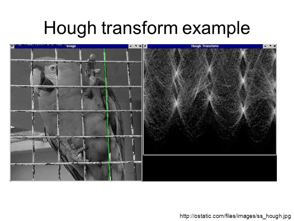
11. Hough transform example

12. Finding lines using Hough transform
Using m,b parameterization
Using r, theta parameterization
Using oriented gradients
Practical considerations
Bin size
Smoothing
Finding multiple lines
Finding line segments

13. Hough transform conclusions
Good
Robust to outliers: each point votes separately
Fairly efficient (much faster than trying all sets of parameters)
Provides multiple good fits
Bad
Some sensitivity to noise
Bin size trades off between noise tolerance, precision, and speed/memory
Can be hard to find sweet spot
Not suitable for more than a few parameters
grid size grows exponentially
Common applications
Line fitting (also circles, ellipses, etc.)
Object instance recognition (parameters are affine transform)
Object category recognition (parameters are position/scale)

14. How would we find circles?
Hough Transform
How would we find circles?
Of fixed radius
Of unknown radius

15. RANSAC Model parameters such that: (RANdom SAmple Consensus) :
Learning technique to estimate
parameters of a model by random
sampling of observed data
Fischler & Bolles in ‘81.
Let me give you an intuition of what is going on. Suppose we have the standard line fitting problem in presence of outliers.
We can formulate this problem as follows: want to find the best partition of points in inlier set and outlier set such that…
The objective consists of adjusting the parameters of a model function so as to best fit a data set.
"best" is defined by a function f that needs to be minimized.
Such that the best parameter of fitting the line give rise to a residual error lower that delta
as when the sum, S, of squared residuals
Model parameters
such that:
Source: Savarese

16. (RANdom SAmple Consensus) :
RANSAC
(RANdom SAmple Consensus) :
Fischler & Bolles in ‘81.
Let me give you an intuition of what is going on. Suppose we have the standard line fitting problem in presence of outliers.
We can formulate this problem as follows: want to find the best partition of points in inlier set and outlier set such that…
The objective consists of adjusting the parameters of a model function so as to best fit a data set.
"best" is defined by a function f that needs to be minimized.
Such that the best parameter of fitting the line give rise to a residual error lower that delta
as when the sum, S, of squared residuals
Algorithm:
Sample (randomly) the number of points required to fit the model
Solve for model parameters using samples
Score by the fraction of inliers within a preset threshold of the model
Repeat 1-3 until the best model is found with high confidence

17. RANSAC Algorithm: Line fitting example
Let me give you an intuition of what is going on. Suppose we have the standard line fitting problem in presence of outliers.
We can formulate this problem as follows: want to find the best partition of points in inlier set and outlier set such that…
The objective consists of adjusting the parameters of a model function so as to best fit a data set.
"best" is defined by a function f that needs to be minimized.
Such that the best parameter of fitting the line give rise to a residual error lower that delta
as when the sum, S, of squared residuals
Algorithm:
Sample (randomly) the number of points required to fit the model (#=2)
Solve for model parameters using samples
Score by the fraction of inliers within a preset threshold of the model
Repeat 1-3 until the best model is found with high confidence
Illustration by Savarese

18. RANSAC Algorithm: Line fitting example
Let me give you an intuition of what is going on. Suppose we have the standard line fitting problem in presence of outliers.
We can formulate this problem as follows: want to find the best partition of points in inlier set and outlier set such that…
The objective consists of adjusting the parameters of a model function so as to best fit a data set.
"best" is defined by a function f that needs to be minimized.
Such that the best parameter of fitting the line give rise to a residual error lower that delta
as when the sum, S, of squared residuals
Algorithm:
Sample (randomly) the number of points required to fit the model (#=2)
Solve for model parameters using samples
Score by the fraction of inliers within a preset threshold of the model
Repeat 1-3 until the best model is found with high confidence

19. RANSAC Algorithm: Line fitting example
Let me give you an intuition of what is going on. Suppose we have the standard line fitting problem in presence of outliers.
We can formulate this problem as follows: want to find the best partition of points in inlier set and outlier set such that…
The objective consists of adjusting the parameters of a model function so as to best fit a data set.
"best" is defined by a function f that needs to be minimized.
Such that the best parameter of fitting the line give rise to a residual error lower that delta
as when the sum, S, of squared residuals
Algorithm:
Sample (randomly) the number of points required to fit the model (#=2)
Solve for model parameters using samples
Score by the fraction of inliers within a preset threshold of the model
Repeat 1-3 until the best model is found with high confidence

20. RANSAC
Let me give you an intuition of what is going on. Suppose we have the standard line fitting problem in presence of outliers.
We can formulate this problem as follows: want to find the best partition of points in inlier set and outlier set such that…
The objective consists of adjusting the parameters of a model function so as to best fit a data set.
"best" is defined by a function f that needs to be minimized.
Such that the best parameter of fitting the line give rise to a residual error lower that delta
as when the sum, S, of squared residuals
Algorithm:
Sample (randomly) the number of points required to fit the model (#=2)
Solve for model parameters using samples
Score by the fraction of inliers within a preset threshold of the model
Repeat 1-3 until the best model is found with high confidence

21. How to choose parameters?
Number of samples N
Choose N so that, with probability p, at least one random sample is free from outliers (e.g. p=0.99) (outlier ratio: e )
Number of sampled points s
Minimum number needed to fit the model
Distance threshold 
Choose  so that a good point with noise is likely (e.g., prob=0.95) within threshold
Zero-mean Gaussian noise with std. dev. σ: t2=3.84σ2
proportion of outliers e s 5%
10%
20%
25%
30%
40%
50% 2 3 5 6 7 11 17 4 9 19 35 13 34 72 12 26 57
146 16 24 37 97
293 8 20 33 54
163
588 44 78
272
1177
modified from M. Pollefeys

22. RANSAC conclusions Good Bad Common applications Robust to outliers
Applicable for larger number of objective function parameters than Hough transform
Optimization parameters are easier to choose than Hough transform
Bad
Computational time grows quickly with fraction of outliers and number of parameters
Not good for getting multiple fits
Common applications
Computing a homography (e.g., image stitching)
Estimating fundamental matrix (relating two views)

23. How do we fit the best alignment?

24. Alignment
Alignment: find parameters of model that maps one set of points to another
Typically want to solve for a global transformation that accounts for *most* true correspondences
Difficulties
Noise (typically 1-3 pixels)
Outliers (often 50%)
Many-to-one matches or multiple objects

25. Parametric (global) warping
p = (x,y)
p’ = (x’,y’)
Transformation T is a coordinate-changing machine:
p’ = T(p)
What does it mean that T is global?
Is the same for any point p
can be described by just a few numbers (parameters)
For linear transformations, we can represent T as a matrix
p’ = Tp

26. Common transformations
original
Transformed
aspect
translation
rotation
affine
perspective
Slide credit (next few slides): A. Efros and/or S. Seitz

27. Scaling
Scaling a coordinate means multiplying each of its components by a scalar
Uniform scaling means this scalar is the same for all components:
 2

28. Scaling Non-uniform scaling: different scalars per component:
X  2, Y  0.5

29. Scaling
Scaling operation:
Or, in matrix form:
scaling matrix S

30.  2-D Rotation (x’, y’) (x, y) x’ = x cos() - y sin()
y’ = x sin() + y cos()

31.  2-D Rotation (x’, y’) (x, y) f Polar coordinates… x = r cos (f)
y = r sin (f)
x’ = r cos (f + )
y’ = r sin (f + )
Trig Identity…
x’ = r cos(f) cos() – r sin(f) sin()
y’ = r sin(f) cos() + r cos(f) sin()
Substitute…
x’ = x cos() - y sin()
y’ = x sin() + y cos() 
(x, y)
(x’, y’) f

32. 2-D Rotation This is easy to capture in matrix form:
Even though sin(q) and cos(q) are nonlinear functions of q,
x’ is a linear combination of x and y
y’ is a linear combination of x and y
What is the inverse transformation?
Rotation by –q
For rotation matrices R

33. Basic 2D transformations
Scale
Shear
Rotate
Translate
Affine is any combination of translation, scale, rotation, shear
Affine

34. Affine Transformations
Affine transformations are combinations of
Linear transformations, and
Translations
Properties of affine transformations:
Lines map to lines
Parallel lines remain parallel
Ratios are preserved
Closed under composition or
Ratios of distances along straight lines are preserved

35. Projective Transformations
Projective transformations are combos of
Affine transformations, and
Projective warps
Properties of projective transformations:
Lines map to lines
Parallel lines do not necessarily remain parallel
Ratios are not preserved
Closed under composition
Models change of basis
Projective matrix is defined up to a scale (8 DOF)

36. 2D image transformations (reference table)
Szeliski 2.1

37. Example: solving for translationB1 B2 B3
Given matched points in {A} and {B}, estimate the translation of the object

38. Example: solving for translationB1 B2 B3
(tx, ty)
Least squares solution
Write down objective function
Derived solution
Compute derivative
Compute solution
Computational solution
Write in form Ax=b
Solve using pseudo-inverse or eigenvalue decomposition

39. Example: solving for translationB4 B1 B2 B3
(tx, ty) A4 B5
Problem: outliers
RANSAC solution
Sample a set of matching points (1 pair)
Solve for transformation parameters
Score parameters with number of inliers
Repeat steps 1-3 N times

40. Example: solving for translationB4 B5 B6 A1 A2 A3 B1 B2 B3
(tx, ty) A4 A5 A6
Problem: outliers, multiple objects, and/or many-to-one matches
Hough transform solution
Initialize a grid of parameter values
Each matched pair casts a vote for consistent values
Find the parameters with the most votes
Solve using least squares with inliers

41. Example: solving for translation
(tx, ty)
Problem: no initial guesses for correspondence

42. What if you want to align but have no prior matched pairs?
Hough transform and RANSAC not applicable
Important applications
Medical imaging: match brain scans or contours
Robotics: match point clouds

43. Iterative Closest Points (ICP) Algorithm
Goal: estimate transform between two dense sets of points
Initialize transformation (e.g., compute difference in means and scale)
Assign each point in {Set 1} to its nearest neighbor in {Set 2}
Estimate transformation parameters
e.g., least squares or robust least squares
Transform the points in {Set 1} using estimated parameters
Repeat steps 2-4 until change is very small

44. Example: solving for translation
(tx, ty)
Problem: no initial guesses for correspondence
ICP solution
Find nearest neighbors for each point
Compute transform using matches
Move points using transform
Repeat steps 1-3 until convergence

45. Algorithm Summary Least Squares Fit Robust Least Squares
closed form solution
robust to noise
not robust to outliers
Robust Least Squares
improves robustness to noise
requires iterative optimization
Hough transform
robust to noise and outliers
can fit multiple models
only works for a few parameters (1-4 typically)
RANSAC
works with a moderate number of parameters (e.g, 1-8)
Iterative Closest Point (ICP)
For local alignment only: does not require initial correspondences