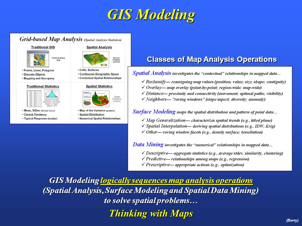
2. GIS Modeling (Berry) GIS Modeling logically sequences map analysis operations (Spatial Analysis, Surface Modeling and Spatial Data Mining) to solve spatial problems… Thinking with Maps Classes of Map Analysis Operations

3. Decision Support Systems Framework (Berry) Three elements of a GIS Model

4. Suitability Modeling (Full Exercise #8) (Berry) Relative Suitability Mountain Property Development

5. Capturing Model Logic (Command Script) The logical sequence of map analysis operations is contained in a Command Script that can be easily changed to simulate different scenarios (Berry)

6. Suitability Modeling (Comparing Scenarios) (Berry)

7. Transmission Line Siting Model Criteria – the transmission line route should… Avoid areas of high housing density Avoid areas of high housing density Avoid areas that are far from roads Avoid areas that are far from roads Avoid areas within or near sensitive areas Avoid areas within or near sensitive areas Avoid areas of high visual exposure to houses Avoid areas of high visual exposure to housesHousesRoads Sensitive Areas Houses Elevation Goal – identify the best route for an electric transmission line that considers various criteria for minimizing adverse impacts. Existing Powerline ProposedSubstation (Berry)

8. Siting Model Flowchart (Model Logic) Model logic is captured in a flowchart where the boxes represent maps and lines identify processing steps leading to a spatial solution High Housing Density Far from Roads In or Near Sensitive Areas High Visual Exposure …build on this single factor Avoid areas of… (Berry)

9. Siting Model Flowchart (Model Logic) Model logic is captured in a flowchart where the boxes represent maps and lines identify processing steps leading to a spatial solution Step 2 Generate an Accumulated Preference surface from the starting location to everywhere Step 2 Start Step 3 Identify the Most Preferred Route from the end location Step 3 End Start Step 1 Identify overall Discrete Preference (1 good to 9 bad rating) Step 1 (Berry)

10. Step 1 Discrete Preference Map (Berry)CalibrationWeighting HDensity RProximity SAreas VExposure

11. Step 2 Accumulated Preference Map (Berry) Splash Algorithm – like tossing a stick into a pond with waves emanating out and accumulating costs as the wave front moves

12. Step 3 Most Preferred Route (Berry) …steepest downhill path “re-traces” the accumulated cost wave front that got there first

13. Generating Optimal Path Corridors (Berry)

14. Power and Pipeline Routing (Advanced GIS Models) Global routing solution identifies the Optimal Route (blue line) and Optimal Corridor (cross-hatched) …see Application Paper \GITA_Oil&Gas_04 Infusing stakeholder perspectives into Calibration and Weighting …of Engineering considerations, Natural Environment consequences and Built Environment impacts …see Application Paper \GW04_routing (Berry)

15. Real World Routing Application (Processing Schematic) B E N B E N (avg) B E N BuiltEngr.Natural Criteria 3) The categories on each Criteria Map are calibrated to a range of 1=best to 9= worst for siting a transmission line Excluded Stakeholder Groups 4) Relative importance weights for the Criteria Maps within each group are used to calculate an overall preference map Categories 2) Information that influence transmission line siting are identified 1) Locations that prohibit siting are eliminated from consideration Exclusions Slope Hydro- graphy Flood- plane Public Lands Existing Utilities Trans- poration Land Cover Proximity Excluded Proximity Buildings etc. Building Density Visual Exposure Proximity Schools Weighting Calibration Simulations 5) The best route and corridor is determined for conditions favoring each group’s perspective and one where all are equally weighted– Four alternative routes reflecting different perspectives (Berry)

16. Identifying the Routing Decision Space Combining alternative corridors identifies the decision space reflecting various perspectives …the routing decision space is identified by combining the Alternative Corridors Weighting one stakeholder group over the others derives Alternative Corridors that emphasize stakeholder particular concerns E=1 N=1 B=5 E=1 N=5 B=1 E=5 N=1 B=1 E=1 N=1 B=1 GeoWorld magazine feature article on the EPRI_GTC project http://www.geoplace.com/gw/2004/0404/0404pwr.asp http://www.geoplace.com/gw/2004/0404/0404pwr.asp

17. Acquire Additional Detailed Field Data The Siting Team collects additional very detailed field data within the decision space defined by the Alternative Corridors

18. Investigating the Alternative Routes (GIS-derived ) Standardized Alternative Routes Built Natural Engineering Simple Less Suitable More Suitable “Simple” Discrete Preference Surface shown as background … avoid areas in warmer tones (red) and favor locating in cooler tones (green) Built-up Area (avoid) Open Field (favor) …based on the detailed field data, the Siting Team investigates the impacts of the Alternative Routes Note: if the additional detailed data warrants, the Siting Team can re-locate portions of the GIS-derived Alternative Routes but a formal statement of the reasons are required; alignment of a potential route outside of the decision space requires an exception petition (analogous to land use re-zoning)

19. Evaluating Potential Routes (selecting the Preferred) …the relative merits of top few potential routes are discussed by the Siting Team and then ranked to identify the most preferred route GIS-derived Scores Expert Judgment

20. The Softer Side of GIS (Beyond Mapping III Epilog) Philosopher's Levels of Understanding Data – all facts Information – facts within a context Knowledge – interrelationships among relevant facts Wisdom – actionable knowledge Prescription  Increasing Abstraction — Description Cognitive Levels of Judgment Facts – Earth circumference is 24,900 mi – Britney Spears was born 12/2/1981 – Britney Spears is 25 years old – the temperature is 32 o F : Relevant Facts – the temperature is 32 o F Perception – it sure is cold (Floridian) – it’s not cold (Alaskan) Opinions/Values – I hate this weather (Floridian) – I love this weather (Alaskan) Map Types Base – measured features, conditions and characteristics (fact) Derived – inferred conditions and characteristics (implied fact) Interpreted – adjusted to reflect expertise and presumption (judgment) Modeled – potential solution within model logic and expression (conjoined judgment) Spatial Processing Collect – direct acquisition of primary information (e.g. elevation) Calculate – uses algorithms to derive secondary information (e.g., slope) Calibrate/Weight – translates information into relative scales (preference & importance) Simulate – “what if” investigation of alternative scenarios (multiple perspectives) Where we have been in GIS Where we are headed in GIS

21. Computer Mapping -- Spatial dB Management -- GIS Modeling Where Have We Been? From mapping to Spatial Reasoning Spatial Reasoning Spatial Analysis — “contextual” relationships within and among mapped Spatial Analysis — “contextual” relationships within and among mapped data (Reclassify, Overlay, Distance, and Neighbors) data (Reclassify, Overlay, Distance, and Neighbors) Data Mining — “numerical” relationships Data Mining — “numerical” relationships within and among mapped data (Descriptive, Predictive, within and among mapped data (Descriptive, Predictive, and Prescriptive) and Prescriptive) Surface Modeling — maps the “spatial distribution” and Surface Modeling — maps the “spatial distribution” and pattern of point data (Map Generalization, Spatial Interpolation pattern of point data (Map Generalization, Spatial Interpolation and Others) and Others) …changing our Map Paradigm Thinking with Maps! (Berry)

22. More on Map Analysis and GIS Modeling (Berry) www.innovativegis.com/basis Software HardcopyBooks OnlinePapersOnlineMaterials