1. 1 Chapters 9 Self-SimilarTraffic

2. Chapter 9 – Self-Similar Traffic 2 Introduction- Motivation Validity of the queuing models we have studied depends on the Poisson nature of data traffic Validity of the queuing models we have studied depends on the Poisson nature of data traffic Recent studies show that Internet traffic patterns are often bursty and self-similar, not Poisson (exponential) Recent studies show that Internet traffic patterns are often bursty and self-similar, not Poisson (exponential) –Patterns appear through time Understanding of the characteristics of self-similar traffic is essential to enable analysis of modern networks Understanding of the characteristics of self-similar traffic is essential to enable analysis of modern networks

3. Chapter 9 – Self-Similar Traffic 3 Introduction- Motivation F(x) = Pr[X  x] = 1 – e - x Exponential Distribution Exponential Density E[X] =  X = 1/ f(x) = F(x) = e - x ddx

4. Chapter 9 – Self-Similar Traffic 4 Sierpinski triangle …can be found …in chaos. Order

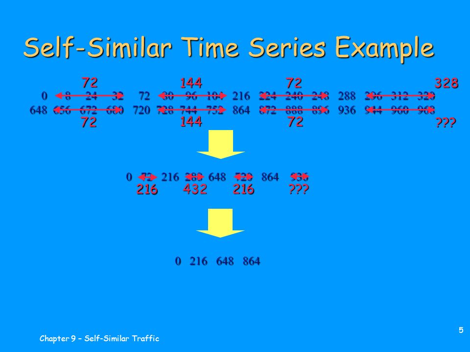
5. Chapter 9 – Self-Similar Traffic 5 Self-Similar Time Series Example 0 8 24 32 72 80 96 104 216 224 240 248 288 296 312 320 0 8 24 32 72 80 96 104 216 224 240 248 288 296 312 320 648 656 672 680 720 728 744 752 864 872 888 896 936 944 960 968 0 72 216 288 648 720 864 936 0 216 648 864 32872144 14472 72 72??? 216 432216 ???

6. Chapter 9 – Self-Similar Traffic 6 Self-Similar Time Series Example Characteristics: Bursty Repeating Pattern independent of scale A phenomenon that is self-similar looks the same or behaves the same when viewed at different degrees of aggregation.

7. Chapter 9 – Self-Similar Traffic 7 Cantor Set – 5 levels of recursion Construction of Cantor Sets: 1. 1.Begin with closed interval [0,1] 2. 2.Remove the open middle third of the interval 3. 3.Repeat for each succeeding interval. Properties: 1. 1.Has structure at arbitrarily small scales 2. 2.The structure repeats These properties do not hold indefinitely, but over a large range of scales, many real phenomena exhibit self-similarity.

8. Chapter 9 – Self-Similar Traffic 8 Relevance in Networking Clustering (a.k.a. burstiness) is common in network traffic patterns Clustering (a.k.a. burstiness) is common in network traffic patterns –patterns are typically persistent through time –the clusters may themselves be clustered Poisson traffic demonstrates clustering in short term, but smoothes over long term (known as the “memoryless” property) Poisson traffic demonstrates clustering in short term, but smoothes over long term (known as the “memoryless” property) During bursts due to clustering, queue sizes in switches/routers may build up more than the classical M/M/1 model predicts During bursts due to clustering, queue sizes in switches/routers may build up more than the classical M/M/1 model predicts –impact on buffer sizes?

9. Chapter 9 – Self-Similar Traffic 9 Relevance in Networking Bottom line - The M/M/1 queuing model assumes that arrivals and service times are exponential and, therefore, “memoryless” … real network traffic patterns might not be memoryless, therefore the M/M/1 model might be “optimistic”

10. Chapter 9 – Self-Similar Traffic 10 Self-Similar Stochastic Processes g(t) is similar to g(t + aT), a = 0,  1,  2, … Less fluctuation, more regularity at longer time scales. g(t) is not similar to g(t + aT), a = 0,  1,  2, …

11. Chapter 9 – Self-Similar Traffic 11 Continuous-Time Self-Similar Stochastic Processes Continuous time: 0  t   Continuous time: 0  t   A stochastic process x(t) is statistically self-similar with parameter H (0.5  H  1), if for a  0: A stochastic process x(t) is statistically self-similar with parameter H (0.5  H  1), if for a  0: a -H x(at) has the same statistical properties as x(t) In other words: In other words:  E[x(t)] = mean  Var[x(t)] = variance  R x (t, s) = autocorrelation E[x(at)] a H Var[x(at)] a 2H R x (at, as) a 2H

12. Chapter 9 – Self-Similar Traffic 12 Hurst Parameter (H) Measure of the persistence of a statistical phenomenon….. the measure of the long-range dependence of a stochastic process Measure of the persistence of a statistical phenomenon….. the measure of the long-range dependence of a stochastic process H = 0.5 indicates absence of long-term dependence H = 0.5 indicates absence of long-term dependence As H approaches 1, the greater the degree of long-term dependence As H approaches 1, the greater the degree of long-term dependence Note: Brownian motion process B(t) is self-similar with H = 0.5 Note: Brownian motion process B(t) is self-similar with H = 0.5 SEE Appendix 9A

13. Chapter 9 – Self-Similar Traffic 13 Heavy-Tailed Distributions It is possible to define self-similar stochastic processes with heavy-tailed distributions It is possible to define self-similar stochastic processes with heavy-tailed distributions Leads to manageable distribution models Leads to manageable distribution models Can be used to characterize probability densities for traffic processes, e.g., packet interarrival times and burst lengths Can be used to characterize probability densities for traffic processes, e.g., packet interarrival times and burst lengths Distribution of random variable X is heavy- tailed if: Distribution of random variable X is heavy- tailed if: 1 – F(x) = Pr[X  x] ~, as x  , 0   1 x 

14. Chapter 9 – Self-Similar Traffic 14 Pareto Heavy-Tailed Distribution Characteristics: Characteristics: f(x) = F(x) = 0 (x  k) f(x) = F(x) = 0 (x  k) F(x) = 1 - (x  k,   0) f(x) = (x  k,   0) E[X] = k (   1) Note that for k = 1, Note that for k = 1,    2, infinite variance    1, infinite mean and variance k  k x k  +1 k  +1x k   -1

15. Chapter 9 – Self-Similar Traffic 15 Pareto and Exponential Examples Density Functions Compared f (x) =  k k x  +1

16. Chapter 9 – Self-Similar Traffic 16 Examples of Self-Similar Data Traffic LAN (Ethernet): LAN (Ethernet): –self-similar, H = 0.9 –Pareto fit for  = 1.2 World-Wide Web: World-Wide Web: –browser traffic nicely fits Pareto distribution for 1.16    1.5 –file sizes on WWW seem to fit this distribution as well TCP - FTP, TELNET: TCP - FTP, TELNET: –session arrivals approximate Poisson –traffic patterns are bursty… heavy-tailed

17. Chapter 9 – Self-Similar Traffic 17 Mean Waiting Time (Delay) – Ethernet/ISDN Study

18. Chapter 9 – Self-Similar Traffic 18 Findings/Implications? Higher loads lead to higher degrees of self- similarity Higher loads lead to higher degrees of self- similarity –performance issues most relevant at high loads Traditional Poisson modeling of traffic proven inadequate Traditional Poisson modeling of traffic proven inadequate –leads to inaccurate queuing analysis results –increased delays, buffer size requirements –applicable to ATM, frame relay, 100BaseT switches, WAN routers, etc. –note excessive cell loss in first generation ATM switches Pareto modeling yields better (more conservative) results Pareto modeling yields better (more conservative) results

19. Chapter 9 – Self-Similar Traffic 19 Self-Similar Modeling (Norros) Attempts to develop reliable analytical model of self-similar behavior Attempts to develop reliable analytical model of self-similar behavior –uses Fractional Brownian Motion (FBM) process (sect. 9.2) as basis Buffer size can often be estimated using: Buffer size can often be estimated using: q =  1/[2(1-H)] / (1-  ) H/(1-H) (note that for H = 0.5, this simplifies to  /(1-  ), the M/M/1 model)

20. Chapter 9 – Self-Similar Traffic 20 Self-Similar Storage Model (Norros)

21. Chapter 9 – Self-Similar Traffic 21 Findings/Implications? Buffer requirements much higher at lower levels of utilization for higher degrees of self- similarity (higher H) Buffer requirements much higher at lower levels of utilization for higher degrees of self- similarity (higher H)THEREFORE… If higher levels of utilization are required, much larger buffers are needed for self- similar traffic than would be predicted using classical modeling If higher levels of utilization are required, much larger buffers are needed for self- similar traffic than would be predicted using classical modeling So, what does all this really mean?

22. Chapter 9 – Self-Similar Traffic 22 Modeling and Estimating Self- Similarity Task: determine if time series of data is actually is self-similar, and estimate the value of H Task: determine if time series of data is actually is self-similar, and estimate the value of H –Variance Time Plot: Var[x (m) ] vs. m –R/S Plot: log[R/S] vs. N –Periodogram: spectral density estimate –Whittle’s Estimator: estimate H, assuming self-similarity