1. Dynamic routing versus static routing Prof. drs. Dr. Leon Rothkrantz http://www.mmi.tudelft.nl http://www.kbs.twi.tudelft.nl

2. Outline presentation Problem definition Static routing Dijkstra shortest path algorithm Dynamic traffic data (historical data, real time data) Dynamic routing using 3D-Dijkstra algorithm Travel speed prediction using ANN Personal intelligent traveling assistant (PITA) PITA in cars and in trains

3. Introduction Problem definition Find the shortest/fastest route from A to B using dynamic route information. Research if dynamic routing results in shorter traveling time compared to shortest path Is it possible to route a traveler on his route in dynamically changing environments ?

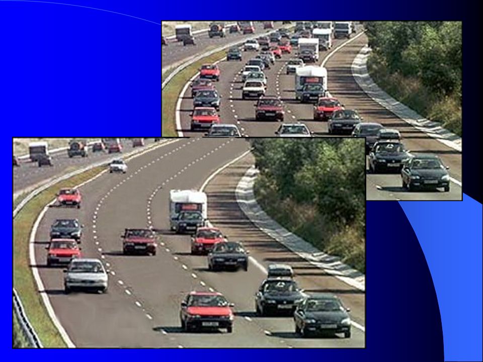
4. (Non-) congested road

5. Traffic

6. Testbed: graph of highways

7. MONICA network Many sensors/wires along the road to measure the speed of the cars

8. Smart Road Many sensors (smart sensors) along a road Sensor devices set up a wireless ad-hoc network Sensor in the car is able to communicate with the road Congestion, icy roads can be detected by the sensors and communicated along the network, to inform drivers remote in place and time GPS, GSM can be included in the sensornetworks Wireless communication by wired lamppost/streetlights

10. Real speed on a road segment during peak hour

11. 3 dimensional graph Use 3D Dijkstra 3 dimensional graph Use 3D Dijkstra

12. Why not search in this 3 dim. graph ? This will become a giant graph: - constructing such a 3 dimensional graph (estimating travel times) would take too much time - performance of shortest path algorithm for such a graph will be very poor

13. Shortest path via dynamic routing

14. Expert system Based on knowledege/experience of daily cardriver (entrance kleinpolderplein ypenburg) (route ypenburg prins_claus) (file prins_claus badhoevedorp) (route badhoevedorp nieuwe_meer) (exit nieuwe_meer coenplein) Translate routes to trajectories between junctions and assign labels entrance, route, file and exit to each trajectory

15. Design (1)

16. Schematic overview of a P+R route.

17. Design (2)

18. Static car and public transport routes

19. Dynamic car route

20. P+R route

21. Expert system (entrance kleinpolderplein ypenburg) (route ypenburg prins_claus) (file prins_claus badhoevedorp) (route badhoevedorp nieuwe_meer) (exit nieuwe_meer coenplein) Translate routes to trajectories between junctions and assign labels entrance, route, file and exit to each trajectory

22. Example alternative routes using expert knowledge

23. Implementation in CLIPS

24. Results of dynamic routing Based on historical traffic speed data dynamic routing is able to save approximately 15% of travel time During special incidents (accidents, road work,…) savings in travel time increases During peak hours savings decreases

25. User preferences Shortest travel time Preference routing via highways, secondary roads minimized Preferred routing (not) via toll routes Fastest route or shortest route Route with minimal of traffic jams

26. Traffic Current systems developed at TUDelft Prediction of travel time using ANN (trained on historical data) Model of speed as function of time average over road segments/trajectories Static routing using Dijkstra algorithm Dynamic routing using 3D Dijkstra Dynamic routing using Ant Based Control algorithm Personal Traveling Assistant online end of 2008

27. NN Classifiers Feed-Forward BP Network – single-frame input – two hidden layers – logistic output function in hidden and output layers – full connections between layers – single output neuron

28. NN Classifiers Time Delayed Neural Network – multiple frames input – coupled weights in first hidden layer for time- dependency learning – logistic output function in hidden and output layers ( continued )

29. NN Classifiers Jordan Recursive Neural Network – single frame input – one hidden layer – logistic output function in hidden and output layer – context neuron for time-dependency learning ( continued )

30. Factors which have impact on the speed Factors Time Day of the week Month Weather Special events

31. Impact on speed Time

32. Impact on speed Day of the week

33. Impact on speed Day of the week

34. Impact on speed Month

35. Impact on speed Month

36. Impact on speed Weather

37. Impact on speed Special events

38. Model 1 Is it possible to predict average speed on a special location and time?

39. Model 1

40. Model 2 Is it possible to predict average time 25 minutes ahead on a special location with an error of less then 10% ?

41. Model 2

42. Model 3

43. Test results Model 1 6 networks tested Tuesday A12 in the direction of Gouda Best results with 5 neurons in hidden layer

44. Test results Model 1

45. Test results Model 2 9 networks tested Tuesday A12 in the direction of Gouda Best results with 9 neurons in the hidden layer

46. Test results Model 2

47. Test results

48. Results of the best performing network: 76% of the values with difference of 10% or less Average error is more than 20% Deleting outliers: average error less than 9%

49. Conclusions Existing research Formula of Fletcher and Goss Impact Results

50. Current system Model (based on historical data) Accidents and work on the road Travel time (based on Recurrent neural networks) Data collection (average speed per segment, per road)

52. Ant Based Control Algorithm (ABC)  Is inspired from the behavior of the real ants  Was designed for routing the data in packet switch networks  Can be applied to any routing problem which assumes dynamic data like:  Routing in mobile Ad-Hoc networks  Dynamic routing of traffic in a city  Evacuation from a dangerous area ( the routing is done to multiple destinations )

53. Natural ants find the shortest route

54. Choosing randomly

55. Laying pheromone

56. Biased choosing

57. 3 reasons for choosing the shortest path Earlier pheromone (trail completed earlier) More pheromone (higher ant density) Younger pheromone (less diffusion)

58. Application of ant behaviour in network management Mobile agents Probability tables Different pheromone for every destination

59. Traffic model in one node ijk 1p i1 p j1 p k1 2p i2 p j2 p k2.. Np iN p jN P kN Routing table Local Traffic Statistics Networknode destinations neighbours 12....N μ 1 ;σ 1 ; W 1 μ 2 ; σ 2 ; W 2 … μ N ; σ N ; W N

60. Routing table To forward the packets, each node has a routing table 6810 1 0.40.50.1 2 0.70.20.1 … 11 0.40.10.5 All possible destinations Neighbours 1 4 2 3 7 9 8 10 11 6 5

61. Generating virtual ants (agents) 1. ants are launched on regular intervals - it goes from source to a randomly chosen destination 1 4 2 1 3 7 9 8 10 11 6 5

62. Chosing the next node 2 1 5 2. Ant chooses its next node according to a probabilistic rule: -probabilities in routing table; -traffic level in the node; 25 110.40.6 neighbours destination

63. 2 Sniffing the network Ant moves towards its destination …and it memories its path 2 11t5t5 10t4t4 9t3t3 3t2t2 2t1t1 1t0t0 11 8 4 3 7 9 11 6 5 3 9 10

64. 2 8 The backward ant Ant goes back using the same path 11t5t5 10t4t4 9t3t3 3t2t2 2t1t1 1t0t0 1 1 11 10 2 4 3 7 9 6 5 3 9

65. Updating the probability tables On its way to the source, ant updates routing tables in all nodes table in 1 before update table after update 25 110.40.6 25 110.80.2 2 8 1 10 1 11 10 2 4 3 7 9 6 5 3 9

66. Simple formulae Calculate reinforcement: Update probabilities:

67. Complex formulae P’ jd =P jd + r(1-P jd ) P’ nd =P nd - rP nd, n<>j

68. Map representation for simulation Simulation environment

69. Results Average trip time for the cars using the routing system Average trip time for the cars that not use the routing system

70. Simulation environment Architecture GPS-satellite Vehicle Routing system Simulation

71. GPS-satellite Vehicle Routing system Position determination Routing Dynamic data Communication flow

72. Routing system Route finding system Memory Timetable updating system Dynamic data Routing

73. 1245… 1 -1215-… 2 11--18… 4 14--13… 5 -1814-… … …………… 1 3 2 4 5 6 7 Routing system (2) Timetable

74. Experiment

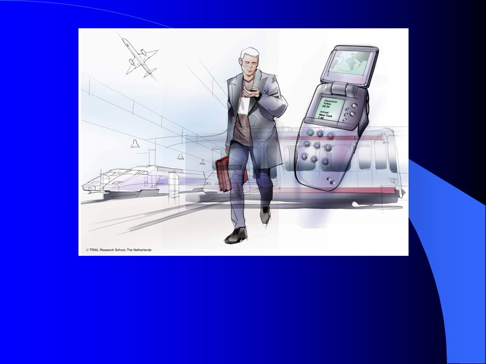
75. Personal intelligent travel assistant PITA is multimodal, speech, touch, text, picture,GPS,GPRS PITA is able to find shortest route in time using dynamic traffic data PITA is able to launch robust agents finding information on different sites (imitating HCI) PITA computes shortest route using AI techniques (expertsystems, case based reasoning, ant based routing alg, adaptive Dijkstra alg.)

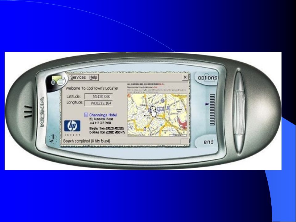
78. PDA

79. Digital Assistant Digital assistant has characteristics of a human operator Ambient Intelligent Context awareness Adaptive to personal characteristics Independent, problem solver Computational, transparent solutions Multimodal input/output

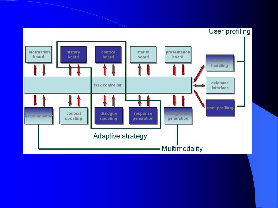
80. Schematic overview of the PITA components

82. Overview of communication Wireless network layers:  human communication layer  virtual communication  virtual coordinating agent

83. Actors, Agents and Services Layers of communication:  overlapping clouds of actors ( human sensors, perception devices)  corresponding clouds of representative agents  clouds of services

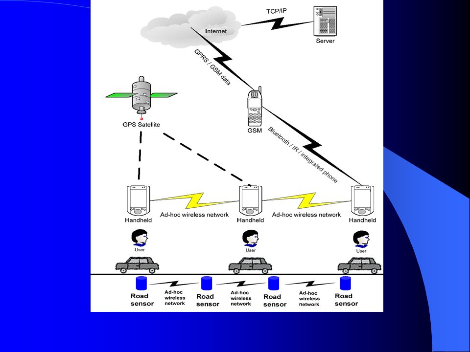
84. Mobile Ad-Hoc Network

85. PITA system in a train Travelers in train have device able to set up a wireless network in the train or to communicate via e-mail, connected to GPS Position of traveler corresponds to position of trains (de-)Centralized systems knows the position of train at every time and is able to reroute and inform travelers in dynamically changing environments

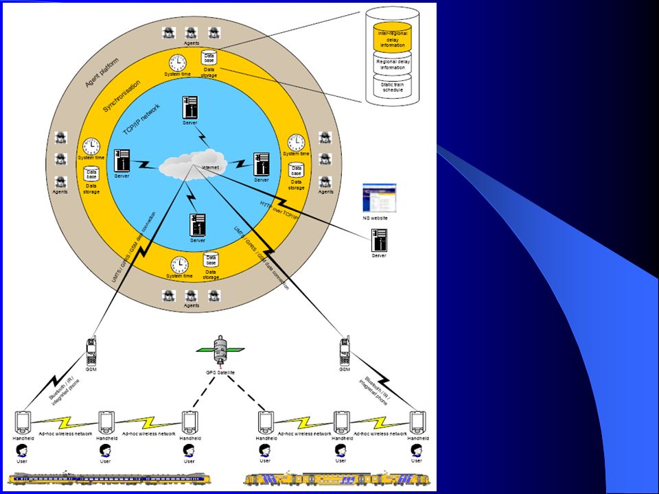
86. A technical view of the PITA system

88. The personal agent

89. The handheld interface model

90. The handheld application model

91. A handheld can be connected to the rest of the system by only an ad-hoc wireless connection

92. Sequence diagram of the addition of a new delay

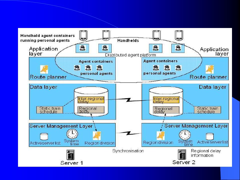
93. The distributed agent platform architecture

98. User profiles THE MAPPING BETWEEN THE USER PROFILES AND THE SEARCH PARAMETERS

99. The route plan to Groningen Noord Search times