1. Sarah Minson Caltech February 22, 2011LLNL

2. Mark Simons (Caltech) James Beck (Caltech)

4. Things we want to know Do regions of co-seismic slip overlap with areas of post-seismic or inter-seismic slip? How do hypocenter locations relate to co-/post- /inter-seismic slip? Do earthquakes have smooth slip distributions and short slip durations? Vice versa? Do earthquakes rupture at super-shear velocities?

5. TeleseismicStrong motionJoint km Delouis et al. (2009) Loveless et al. (2010) Seismic + Static

6. Seismology: To get to earthquake physics, we need better source models Math: Many geophysical problems are under-determined Ill-posed inverse problems require regularization Roughness of the slip distribution (or whatever quantity is being regularized) cannot be identified because it was set a piori.

7. For inverse problems: PosteriorPosteriorPriorPriorDataLikelihoodDataLikelihood

8. OptimizationBayesian One solutionDistribution of solutions Converges to one minimumMulti-peaked solution spaces OK Regularization may be requiredNo a priori regularization required Limited choice of a priori constraintsGeneralized a priori constraints Error analysis hard for nonlinear problemsError analysis comes free with solution Sensitive to model parameterization (model covariance leads to trade-offs) Insensitive to model parameterization (if model covariance is estimated)

9. Calculating posterior PDF generally requires Monte Carlo simulation “Curse of Dimensionality” Huge numbers of samples required for high-dimensional problems Sampling can be inefficient especially in high - dimensional problems

10. Efficient parallel sampling algorithm Metropolis algorithm and Markov Chain Monte Carlo (MCMC) are serial Must efficiently sample highly anti-correlated model parameters Must share information between worker CPUs

11. Tempering (A.K.A. Simulated Annealing) * Dynamic cooling schedule ** Resampling ** Parallel Metropolis Simulation adapts to model covariance ** Simulation adapts to rejection rate *** Cascading * Marinari and Parisi (1992) ** Ching and Chen (2007) *** Matt Muto

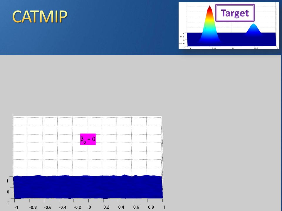
12. 1.Sample P( θ ) 2.Calculate β 3.Resample 4.Metropolis algorithm in parallel 5.Collect final samples 6.Go back to Step 2, lather, rinse, and repeat until cooling is achieved

13. 1.Sample P( θ ) 2.Calculate β 3.Resample 4.Metropolis algorithm in parallel 5.Collect final samples 6.Go back to Step 2, lather, rinse, and repeat until cooling is achieved

16. For each patch on a regularly gridded fault plane Two components of slip Rise time Rupture velocity Also may solve for ramp components of InSAR Total number of parameters: 4*N patches (+ ramp)

17. Slip Rotated coordinate system relative to teleseismic rake direction Slip parallel to rake has a positivity constraint Forbidden from back-slipping more than 1 m Prior distribution on slip perpendicular to rake is a zero- mean Gaussian Prior distribution is populated from Dirichlet distribution Prior distribution on rupture velocity and rise time is uniform

18. d predicted =G*slip

19. Green’s functions are pre-computed These are then convolved with all possible source time durations and stored in memory Convolution is too slow to be done at evaluation time Final predicted waveforms are linear combination of each point source (with the appropriate pre-convolved source-time functions) scaled by slip, time-shifted according to results of Fast Sweeping Fast Sweeping Algorithm (Zhao, 2005) is used to calculate initial rupture time at each source from Vr on each patch Source parameters from each patch are interpolated onto a fine grid of point sources

20. Run parameters: Markov chains = 500,000 Steps per Markov chain = 100 2001 cores on CITerra Beowulf cluster Results: Cooling steps = 39 Forward model evaluations = 1.931 billion Run time = 10.6 hours Total computation time = 76.3 million CPU seconds

21. Each model evaluation = 0.035 sec Static forward model = 0.005 sec Kinematic forward model = 0.03 sec Total model evaluation time = 68 million CPU seconds ~90% of time spent on parallel model evaluation

22. Caltech Center for Advanced Computing Research (CACR) is working on a GPU version of CATMIP Michael Aivazis Martin Michaelson As of now, they have a first cut version with partial utilization of GPU ~35x speed-up relative to CPU version Need to move more of code onto GPU

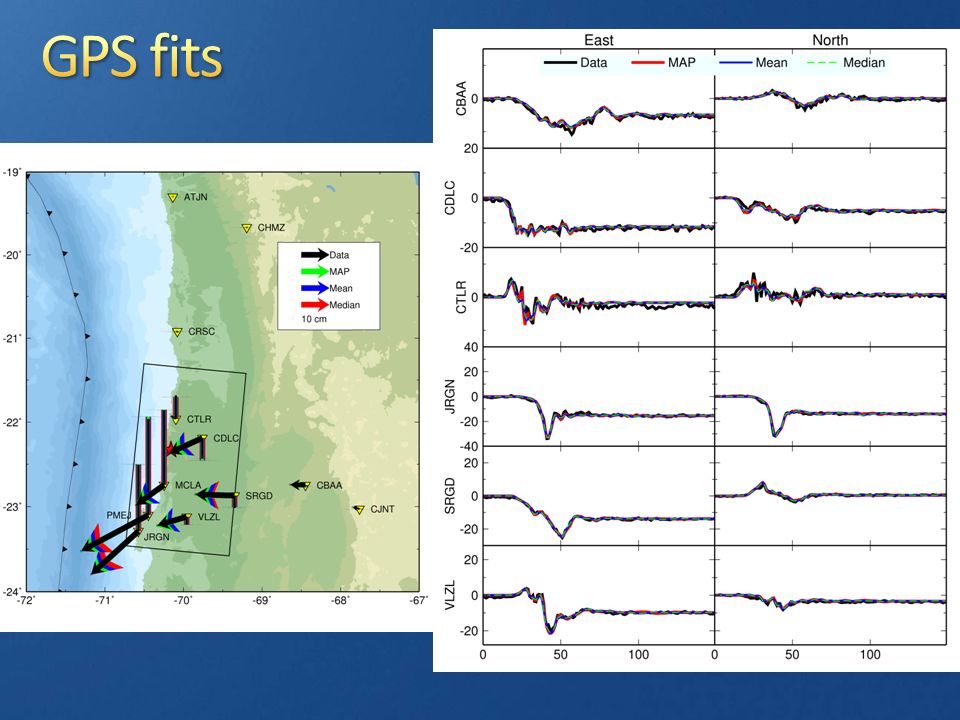
24. Static GPS displacements 1 Hz GPS time series 6 interferograms

25. Static Posterior/ Kinematic Prior Static Posterior/ Kinematic Prior Kinematic Posterior Static Prior

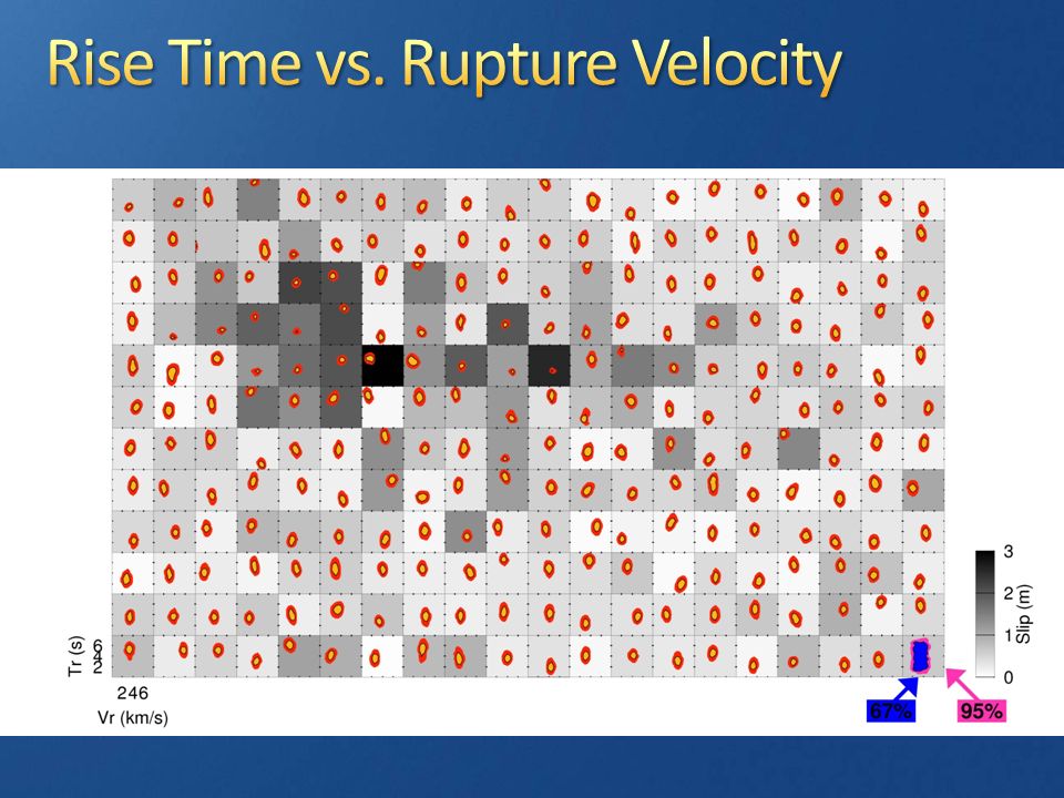
31. U┴U┴U┴U┴ U┴U┴U┴U┴ U║U║U║U║ U║U║U║U║ τrτrτrτr τrτrτrτr VrVrVrVr VrVrVrVr

35. Smoother Rougher

36. VsVs VsVs

37. How do you represent an N-dimensional PDF? People like looking at slip models… …But individual models can be very misleading…

39. MeanMAPMedian

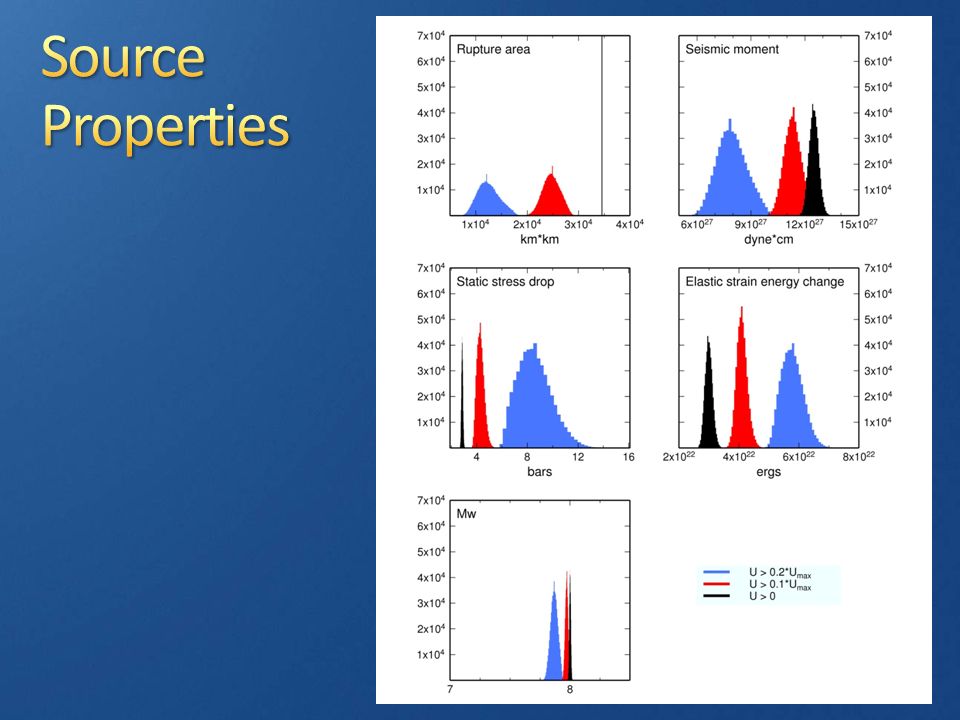
41. CATMIP algorithm allows the sampling of very high-dimensional problems Also useful for low-dimension problems with expensive forward models Wide variety of uses in geophysics Fully Bayesian finite fault earthquake source modeling Resolution of the slip distribution and rupture propagation Uncertainties on derived source properties Determine which source characteristics are constrained and which are not

42. Data errors and model prediction errors are important Assumed data errors control posterior model errors Posterior distribution is also affected by model prediction errors (the failings of the forward model) The next step is to estimate these errors