Theses slides are based on the slides by

Theses slides are based on the slides by
CISC 4631 Data Mining Lecture 07: Naïve Baysean Classifier Theses slides are based on the slides by Tan, Steinbach and Kumar (textbook authors) Eamonn Koegh (UC Riverside) Andrew Moore (CMU/Google)

Naïve Bayes Classifier
Thomas Bayes We will start off with a visual intuition, before looking at the math…

Grasshoppers Katydids 10 1 2 3 4 5 6 7 8 9 Antenna Length
Abdomen Length Remember this example? Let’s get lots more data…

With a lot of data, we can build a histogram
With a lot of data, we can build a histogram. Let us just build one for “Antenna Length” for now… 10 1 2 3 4 5 6 7 8 9 Antenna Length Katydids Grasshoppers

We can leave the histograms as they are, or we can summarize them with two normal distributions.
Let us us two normal distributions for ease of visualization in the following slides…

There is a formal way to discuss the most probable classification…
We want to classify an insect we have found. Its antennae are 3 units long. How can we classify it? We can just ask ourselves, give the distributions of antennae lengths we have seen, is it more probable that our insect is a Grasshopper or a Katydid. There is a formal way to discuss the most probable classification… p(cj | d) = probability of class cj, given that we have observed d 3 Antennae length is 3

p(cj | d) = probability of class cj, given that we have observed d
P(Grasshopper | 3 ) = 10 / (10 + 2) = 0.833 P(Katydid | 3 ) = 2 / (10 + 2) = 0.166 10 2 3 Antennae length is 3

Bayes Classifiers That was a visual intuition for a simple case of the Bayes classifier, also called: Idiot Bayes Naïve Bayes Simple Bayes We are about to see some of the mathematical formalisms, and more examples, but keep in mind the basic idea. Find out the probability of the previously unseen instance belonging to each class, then simply pick the most probable class.

Bayesian Classifiers Bayesian classifiers use Bayes theorem, which says p(cj | d ) = p(d | cj ) p(cj) p(d) p(cj | d) = probability of instance d being in class cj, This is what we are trying to compute p(d | cj) = probability of generating instance d given class cj, We can imagine that being in class cj, causes you to have feature d with some probability p(cj) = probability of occurrence of class cj, This is just how frequent the class cj, is in our database p(d) = probability of instance d occurring This can actually be ignored, since it is the same for all classes

Bayesian Classifiers Given a record with attributes (A1, A2,…,An)
The goal is to predict class C Actually, we want to find the value of C that maximizes P(C| A1, A2,…,An ) Can we estimate P(C| A1, A2,…,An ) directly (w/o Bayes)? Yes, we simply need to count up the number of times we see A1, A2,…,An and then see what fraction belongs to each class For example, if n=3 and the feature vector “4,3,2” occurs 10 times and 4 of these belong to C1 and 6 to C2, then: What is P(C1|”4,3,2”)? What is P(C2|”4,3,2”)? Unfortunately, this is generally not feasible since not every feature vector will be found in the training set (remember the crime scene analogy from the previous lecture?)

Bayesian Classifiers Indirect Approach: Use Bayes Theorem
compute the posterior probability P(C | A1, A2, …, An) for all values of C using the Bayes theorem Choose value of C that maximizes P(C | A1, A2, …, An) Equivalent to choosing value of C that maximizes P(A1, A2, …, An|C) P(C) Since the denominator is the same for all values of C

How can we estimate P(A1, A2, …, An |C)? We can measure it directly, but only if the training set samples every feature vector. Not practical! So, we must assume independence among attributes Ai when class is given: P(A1, A2, …, An |C) = P(A1| Cj) P(A2| Cj)… P(An| Cj) Then we can estimate P(Ai| Cj) for all Ai and Cj from training data This is reasonable because now we are looking only at one feature at a time. We can expect to see each feature value represented in the training data. New point is classified to Cj if P(Cj)  P(Ai| Cj) is maximal.

c1 = male, and c2 = female. Assume that we have two classes
We have a person whose sex we do not know, say “drew” or d. Classifying drew as male or female is equivalent to asking is it more probable that drew is male or female, I.e which is greater p(male | drew) or p(female | drew) (Note: “Drew can be a male or female name”) Drew Barrymore Drew Carey What is the probability of being called “drew” given that you are a male? What is the probability of being a male? p(male | drew) = p(drew | male ) p(male) p(drew) What is the probability of being named “drew”? (actually irrelevant, since it is that same for all classes)

p(cj | d) = p(d | cj ) p(cj) p(d)
This is Officer Drew (who arrested me in 1997). Is Officer Drew a Male or Female? Luckily, we have a small database with names and sex. We can use it to apply Bayes rule… Name Sex Drew Male Claudia Female Alberto Karin Nina Sergio Officer Drew p(cj | d) = p(d | cj ) p(cj) p(d)

p(cj | d) = p(d | cj ) p(cj) p(d)
Name Sex Drew Male Claudia Female Alberto Karin Nina Sergio p(cj | d) = p(d | cj ) p(cj) p(d) Officer Drew p(male | drew) = 1/3 * 3/8 = 0.125 3/ /8 Officer Drew is more likely to be a Female. p(female | drew) = 2/5 * 5/8 = 0.250 3/ /8

Officer Drew IS a female!
So far we have only considered Bayes Classification when we have one attribute (the “antennae length”, or the “name”). But we may have many features. How do we use all the features? Officer Drew p(male | drew) = 1/3 * 3/8 = 0.125 3/ /8 p(female | drew) = 2/5 * 5/8 = 0.250 3/ /8

p(cj | d) = p(d | cj ) p(cj) p(d)
Name Over 170CM Eye Hair length Sex Drew No Blue Short Male Claudia Yes Brown Long Female Alberto Karin Nina Sergio

p(d|cj) = p(d1|cj) * p(d2|cj) * ….* p(dn|cj)
To simplify the task, naïve Bayesian classifiers assume attributes have independent distributions, and thereby estimate p(d|cj) = p(d1|cj) * p(d2|cj) * ….* p(dn|cj) The probability of class cj generating instance d, equals…. The probability of class cj generating the observed value for feature 1, multiplied by.. The probability of class cj generating the observed value for feature 2, multiplied by..

cj … Naïve Bayes is fast and space efficient
We can look up all the probabilities with a single scan of the database and store them in a (small) table… … p(d1|cj) p(d2|cj) p(dn|cj) Sex Over190cm Male Yes 0.15 No 0.85 Female 0.01 0.99 Sex Long Hair Male Yes 0.05 No 0.95 Female 0.70 0.30 Sex Male Female

Naïve Bayes is NOT sensitive to irrelevant features...
Suppose we are trying to classify a persons sex based on several features, including eye color. (Of course, eye color is completely irrelevant to a persons gender) p(Jessica |cj) = p(eye = brown|cj) * p( wears_dress = yes|cj) * …. p(Jessica | Female) = 9,000/10, * 9,975/10,000 * …. p(Jessica | Male) = 9,001/10, * 2/10, * …. Almost the same! However, this assumes that we have good enough estimates of the probabilities, so the more data the better.

cj … p(d1|cj) p(d2|cj) p(dn|cj)
An obvious point. I have used a simple two class problem, and two possible values for each example, for my previous examples. However we can have an arbitrary number of classes, or feature values … p(d1|cj) p(d2|cj) p(dn|cj) Animal Color Cat Black 0.33 White 0.23 Brown 0.44 Dog 0.97 0.03 0.90 Pig 0.04 0.01 0.95 Animal Cat Dog Pig Animal Mass >10kg Cat Yes 0.15 No 0.85 Dog 0.91 0.09 Pig 0.99 0.01

Naïve Bayesian Classifier
Problem! Naïve Bayes assumes independence of features… p(d|cj) Naïve Bayesian Classifier p(d1|cj) p(d2|cj) p(dn|cj) Sex Over 6 foot Male Yes 0.15 No 0.85 Female 0.01 0.99 Sex Over 200 pounds Male Yes 0.11 No 0.80 Female 0.05 0.95

Solution Consider the relationships between attributes… p(d|cj) Naïve Bayesian Classifier p(d1|cj) p(d2|cj) p(dn|cj) Sex Over 6 foot Male Yes 0.15 No 0.85 Female 0.01 0.99 Sex Over 200 pounds Male Yes and Over 6 foot 0.11 No and Over 6 foot 0.59 Yes and NOT Over 6 foot 0.05 No and NOT Over 6 foot 0.35 Female 0.01

Solution Consider the relationships between attributes… p(d|cj) Naïve Bayesian Classifier p(d1|cj) p(d2|cj) p(dn|cj) But how do we find the set of connecting arcs??

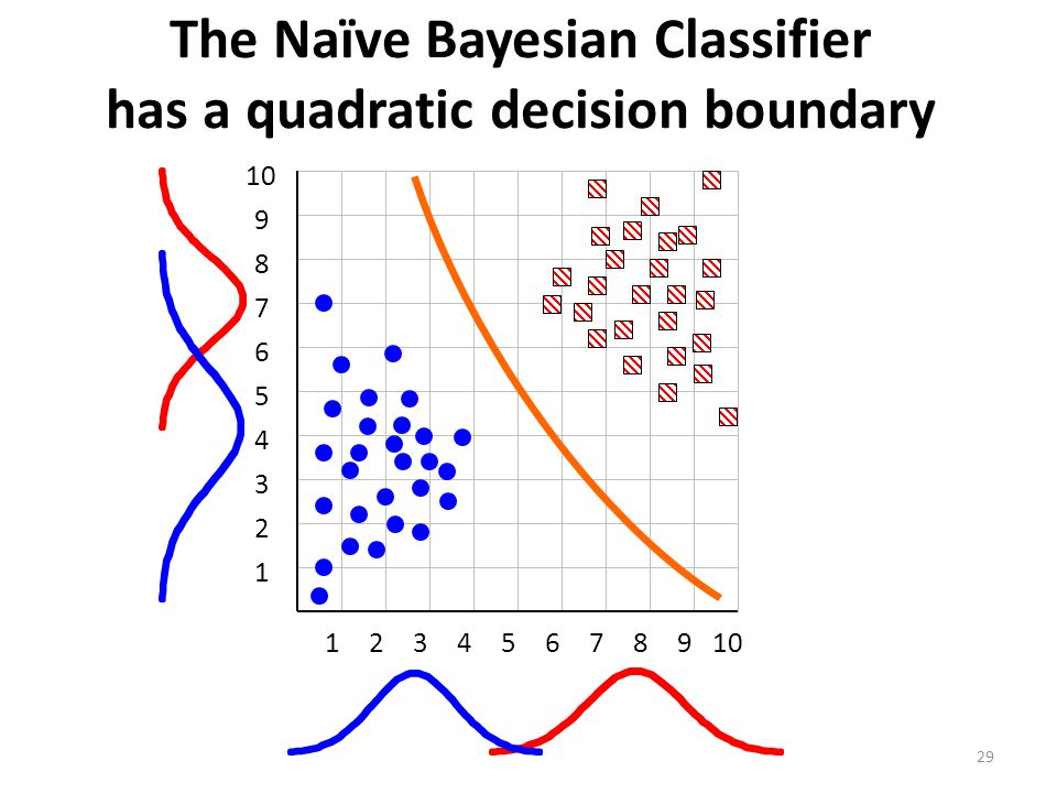
The Naïve Bayesian Classifier has a quadratic decision boundary
10 1 2 3 4 5 6 7 8 9

How to Estimate Probabilities from Data?
For continuous attributes: Discretize the range into bins Two-way split: (A < v) or (A > v) choose only one of the two splits as new attribute Creates a binary feature Probability density estimation: Assume attribute follows a normal distribution and use the data to fit this distribution Once probability distribution is known, can use it to estimate the conditional probability P(Ai|c) We will not deal with continuous values on HW or exam Just understand the general ideas above For the example tax cheating example, we will assume that “Taxable Income” is discrete Each of the 10 values will therefore have a prior probability of 1/10 k

Example of Naïve Bayes We start with a test example and want to know its class. Does this individual evade their taxes: Yes or No? Here is the feature vector: Refund = No, Married, Income = 120K Now what do we do? First try writing out the thing we want to measure

Example of Naïve Bayes We start with a test example and want to know its class. Does this individual evade their taxes: Yes or No? Here is the feature vector: Refund = No, Married, Income = 120K Now what do we do? First try writing out the thing we want to measure P(Evade|[No, Married, Income=120K]) Next, what do we need to maximize?

Example of Naïve Bayes We start with a test example and want to know its class. Does this individual evade their taxes: Yes or No? Here is the feature vector: Refund = No, Married, Income = 120K Now what do we do? First try writing out the thing we want to measure P(Evade|[No, Married, Income=120K]) Next, what do we need to maximize? P(Cj)  P(Ai| Cj)

Example of Naïve Bayes Since we want to maximize P(Cj)  P(Ai| Cj)
What quantities do we need to calculate in order to use this equation? Someone come up to the board and write them out, without calculating them Recall that we have three attributes: Refund: Yes, No Marital Status: Single, Married, Divorced Taxable Income: 10 different “discrete” values While we could compute every P(Ai| Cj) for all Ai, we only need to do it for the attribute values in the test example

Values to Compute Given we need to compute P(Cj)  P(Ai| Cj)
We need to compute the class probabilities P(Evade=No) P(Evade=Yes) We need to compute the conditional probabilities P(Refund=No|Evade=No) P(Refund=No|Evade=Yes) P(Marital Status=Married|Evade=No) P(Marital Status=Married|Evade=Yes) P(Income=120K|Evade=No) P(Income=120K|Evade=Yes)

Computed Values Given we need to compute P(Cj)  P(Ai| Cj)
We need to compute the class probabilities P(Evade=No) = 7/10 = .7 P(Evade=Yes) = 3/10 = .3 We need to compute the conditional probabilities P(Refund=No|Evade=No) = 4/7 P(Refund=No|Evade=Yes) 3/3 = 1.0 P(Marital Status=Married|Evade=No) = 4/7 P(Marital Status=Married|Evade=Yes) =0/3 = 0 P(Income=120K|Evade=No) = 1/7 P(Income=120K|Evade=Yes) = 0/7 = 0

Finding the Class Now compute P(Cj)  P(Ai| Cj) for both classes for the test example [No, Married, Income = 120K] For Class Evade=No we get: .7 x 4/7 x 4/7 x 1/7 = 0.032 For Class Evade=Yes we get: .3 x 1 x 0 x 0 = 0 Which one is best? Clearly we would select “No” for the class value Note that these are not the actual probabilities of each class, since we did not divide by P([No, Married, Income = 120K])

If one of the conditional probability is zero, then the entire expression becomes zero This is not ideal, especially since probability estimates may not be very precise for rarely occurring values We use the Laplace estimate to improve things. Without a lot of observations, the Laplace estimate moves the probability towards the value assuming all classes equally likely Solution  smoothing

Smoothing To account for estimation from small samples, probability estimates are adjusted or smoothed. Laplace smoothing using an m-estimate assumes that each feature is given a prior probability, p, that is assumed to have been previously observed in a “virtual” sample of size m. For binary features, p is simply assumed to be 0.5.

Laplace Smothing Example
Assume training set contains 10 positive examples: 4: small 0: medium 6: large Estimate parameters as follows (if m=1, p=1/3) P(small | positive) = (4 + 1/3) / (10 + 1) = P(medium | positive) = (0 + 1/3) / (10 + 1) = 0.03 P(large | positive) = (6 + 1/3) / (10 + 1) = P(small or medium or large | positive) =

Continuous Attributes
If Xi is a continuous feature rather than a discrete one, need another way to calculate P(Xi | Y). Assume that Xi has a Gaussian distribution whose mean and variance depends on Y. During training, for each combination of a continuous feature Xi and a class value for Y, yk, estimate a mean, μik , and standard deviation σik based on the values of feature Xi in class yk in the training data. During testing, estimate P(Xi | Y=yk) for a given example, using the Gaussian distribution defined by μik and σik .

Naïve Bayes (Summary) Robust to isolated noise points
Robust to irrelevant attributes Independence assumption may not hold for some attributes But works surprisingly well in practice for many problems

More Examples There are two more examples coming up
Go over them before trying the HW, unless you are clear on Bayesian Classifiers You are not responsible for Bayesian Belief Networks

Example of Naïve Bayes Classifier
A: attributes M: mammals N: non-mammals P(A|M)P(M) > P(A|N)P(N) => Mammals

Computer Example: Data Table
Rec Age Income Student Credit_rating Buys_computer 1 <=30 High No Fair 2 Excellent 3 31..40 Yes 4 >40 Medium 5 Low 6 7 8 9 10 11 12 13 14

Computer Example I am 35-year old I earn $40,000 My credit rating is fair Will he buy a computer? X : 35 years old customer with an income of $40,000 and fair credit rating. H : Hypothesis that the customer will buy a computer.

Bayes Theorem P(H|X) : Probability that the customer will buy a computer given that we know his age, credit rating and income. (Posterior Probability of H) P(H) : Probability that the customer will buy a computer regardless of age, credit rating, income (Prior Probability of H) P(X|H) : Probability that the customer is 35 yrs old, have fair credit rating and earns $40,000, given that he has bought our computer (Posterior Probability of X) P(X) : Probability that a person from our set of customers is 35 yrs old, have fair credit rating and earns $40,000. (Prior Probability of X)

Computer Example: Description
The data samples are described by attributes age, income, student, and credit. The class label attribute, buy, tells whether the person buys a computer, has two distinct values, yes (Class C1) and no (Class C2). The sample we wish to classify is X = (age <= 30, income = medium, student = yes, credit = fair) We need to maximize P(X|Ci)P(Ci), for i = 1, 2. P(Ci), the a priori probability of each class, can be estimated based on the training samples:

X = (age <= 30, income = medium, student = yes, credit = fair) To compute P(X|Ci), for i = 1, 2, we compute the following conditional probabilities:

X = (age <= 30, income = medium, student = yes, credit = fair) Using probabilities from the two previous slides:

Tennis Example 2: Data Table
Rec Outlook Temperature Humidity Wind PlayTannis 1 Sunny Hot High Weak No 2 Strong 3 Overcast Yes 4 Rain Mild 5 Cool Normal 6 7 8 9 10 11 12 13 14

Tennis Example 2: Description
The data samples are described by attributes outlook, temperature, humidity and wind. The class label attribute, PlayTennis, tells whether the person will play tennis or not, has two distinct values, yes (Class C1) and no (Class C2). The sample we wish to classify is X = (outlook=sunny, temperature=cool, humidity = high, wind=strong) We need to maximize P(X|Ci)P(Ci), for i = 1, 2. P(Ci), the a priori probability of each class, can be estimated based on the training samples:

X = (outlook=sunny, temperature=cool, humidity = high, wind=strong) To compute P(X|Ci), for i = 1, 2, we compute the following conditional probabilities:

X = (outlook=sunny, temperature=cool, humidity = high, wind=strong) Using probabilities from the previous two pages we can compute the probability in question: hMAP is not playing tennis Normalization:

Dear SIR, I am Mr. John Coleman and my sister is Miss Rose Colemen, we are the children of late Chief Paul Colemen from Sierra Leone. I am writing you in absolute confidence primarily to seek your assistance to transfer our cash of twenty one Million Dollars ($21, ) now in the custody of a private Security trust firm in Europe the money is in trunk boxes deposited and declared as family valuables by my late father as a matter of fact the company does not know the content as money, although my father made them to under stand that the boxes belongs to his foreign partner. …

This mail is probably spam
This mail is probably spam. The original message has been attached along with this report, so you can recognize or block similar unwanted mail in future. See for more details. Content analysis details: (12.20 points, 5 required) NIGERIAN_SUBJECT2 (1.4 points) Subject is indicative of a Nigerian spam FROM_ENDS_IN_NUMS (0.7 points) From: ends in numbers MIME_BOUND_MANY_HEX (2.9 points) Spam tool pattern in MIME boundary URGENT_BIZ (2.7 points) BODY: Contains urgent matter US_DOLLARS_ (1.5 points) BODY: Nigerian scam key phrase ($NN,NNN,NNN.NN) DEAR_SOMETHING (1.8 points) BODY: Contains 'Dear (something)' BAYES_ (1.6 points) BODY: Bayesian classifier says spam probability is 30 to 40% [score: ] Naïve Bayesian is a standard classifier to distinguish between spam and non-spam

Bayesian Classification
Statistical method for classification. Supervised Learning Method. Assumes an underlying probabilistic model, the Bayes theorem. Can solve diagnostic and predictive problems. Can solve problems involving both categorical and continuous valued attributes. Particularly suited when the dimensionality of the input is high In spite of the over-simplified assumption, it often performs better in many complex real-world situations Advantage: Requires a small amount of training data to estimate the parameters

Advantages/Disadvantages of Naïve Bayes
Fast to train (single scan). Fast to classify Not sensitive to irrelevant features Handles real and discrete data Handles streaming data well Disadvantages: Assumes independence of features

Theses slides are based on the slides by

Similar presentations

Presentation on theme: "Theses slides are based on the slides by"— Presentation transcript:

Similar presentations

About project

Feedback

Log in

Auth with social network:

Theses slides are based on the slides by

Similar presentations

Presentation on theme: "Theses slides are based on the slides by"— Presentation transcript:

Similar presentations

About project

Feedback