Download presentation
Presentation is loading. Please wait.

1
Finite Impuse Response Filters

2
Filters A filter is a system that processes a signal in some desired fashion. –A continuous-time signal or continuous signal of x(t) is a function of the continuous variable t. A continuous-time signal is often called an analog signal. –A discrete-time signal or discrete signal x(kT) is defined only at discrete instances t=kT, where k is an integer and T is the uniform spacing or period between samples
 is a function of the continuous variable t. A continuous-time signal is often called an analog signal. –A discrete-time signal or discrete signal x(kT) is defined only at discrete instances t=kT, where k is an integer and T is the uniform spacing or period between samples.")
5
Types of Filters There are two broad categories of filters: –An analog filter processes continuous-time signals –A digital filter processes discrete-time signals. The analog or digital filters can be subdivided into four categories: –Lowpass Filters –Highpass Filters –Bandstop Filters –Bandpass Filters

6
Ideal Filters PassbandStopband Passband Stopband Lowpass FilterHighpass Filter Bandstop Filter PassbandStopband Bandpass Filter M( ) c c c 1 c 1 c 2 c 2
 c c c 1 c 1 c 2 c 2")
7
Discrete-Time Signals Discrete-Time System T{ } x[n] y[n]=T{x[n]} inputoutput The diagram suggests that the output sequence is related to the input sequence by a process that can be described mathematically by an operator T.
![Discrete-Time Signals Discrete-Time System T{ } x[n] y[n]=T{x[n]} inputoutput The diagram suggests that the output sequence is related to the input sequence by a process that can be described mathematically by an operator T.](http://images.slideplayer.com/18/6166400/slides/slide_7.jpg "Discrete-Time Signals Discrete-Time System T{ } x[n] y[n]=T{x[n]} inputoutput The diagram suggests that the output sequence is related to the input sequence by a process that can be described mathematically by an operator T.")
8
Moving Average Filter A simple, but useful filter is the moving average filter. Assume we have the following inputs, x[n]: 2 4 6

9
A 3-point average for a finite-length signal of the values {x[0], x[1], x[2]} = {2, 4, 6} gives the answer ⅓ (2+4+6) = 4. This value defines one of the output values. The next output value is obtained by averaging {x[1], x[2], x[3]} = {4, 6, 4} that yields a value of 14/3.
![A 3-point average for a finite-length signal of the values {x[0], x[1], x[2]} = {2, 4, 6} gives the answer ⅓ (2+4+6) = 4.](http://images.slideplayer.com/18/6166400/slides/slide_9.jpg "This value defines one of the output values. The next output value is obtained by averaging {x[1], x[2], x[3]} = {4, 6, 4} that yields a value of 14/3..")
10
y[0] = ⅓(x[0] + x[1] + x[2]) y[1] = ⅓ (x[1] + x[2] + x[3]) which generalizes to the following input-output equation y[n] = ⅓ (x[n] + x[n+1] + x[n+2]) This equation is called a difference equation.
![y[0] = ⅓(x[0] + x[1] + x[2]) y[1] = ⅓ (x[1] + x[2] + x[3]) which generalizes to the following input-output equation y[n] = ⅓ (x[n] + x[n+1] + x[n+2]) This equation is called a difference equation.](http://images.slideplayer.com/18/6166400/slides/slide_10.jpg "y[0] = ⅓(x[0] + x[1] + x[2]) y[1] = ⅓ (x[1] + x[2] + x[3]) which generalizes to the following input-output equation y[n] = ⅓ (x[n] + x[n+1] + x[n+2]) This equation is called a difference equation.")
11
For the triangular input, the result is the signal y[n] as tabulated below: Note that the values bold type in the x[n] row are the numbers involved in the computation of y[2].
![For the triangular input, the result is the signal y[n] as tabulated below: Note that the values bold type in the x[n] row are the numbers involved in the computation of y[2].](http://images.slideplayer.com/18/6166400/slides/slide_11.jpg "For the triangular input, the result is the signal y[n] as tabulated below: Note that the values bold type in the x[n] row are the numbers involved in the computation of y[2].")
12
The output sequence is plotted below: 2 4 6 Note that the output sequence is longer than the input sequence and somewhat rounded.

13
In general, values from either the present or future or both can be used FIR filter calculations. A filter that uses only the present and past values of the input is called a causal filter. A filter that uses future values of the input is called a non-causal filter. An alternative output indexing scheme can produce a filter that is causal.

14
For the previous problem, the output becomes: Note that this form is simply a time-shifted form of the original form.

15
The General FIR Filter The general form for the FIR filter is:

16
Implementation of FIR Filters Recall that the general form for the FIR filter is:

17
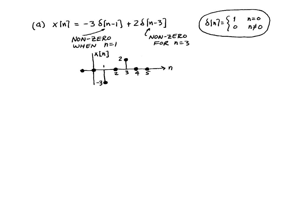
The Unit Impulse The unit impulse is perhaps the simplest sequence because it has only one non-zero value, which occurs at t = 0. The mathematical notation is: 1

18
The Shifted Impulse 1 k The shifted impulse, [n-k], is non-zero when its argument is zero, i.e., n-k = 0, or when n = 0.
![The Shifted Impulse 1 k The shifted impulse, [n-k], is non-zero when its argument is zero, i.e., n-k = 0, or when n = 0.](http://images.slideplayer.com/18/6166400/slides/slide_18.jpg "The Shifted Impulse 1 k The shifted impulse, [n-k], is non-zero when its argument is zero, i.e., n-k = 0, or when n = 0.")
19
The shifted impulse is a very useful concept for representing signals and systems. For example, 2 4 6

20
In order to implement this form, we need the following: (1) a means of multiplying delayed-input signals by the filter coefficients; (2) a means of adding the scaled sequence values; (3) a means of obtaining delayed versions of the input sequence.
 a means of multiplying delayed-input signals by the filter coefficients; (2) a means of adding the scaled sequence values; (3) a means of obtaining delayed versions of the input sequence.")
21
It is useful to represent these operations in block diagram form. × x[n]y[n] y[n] = x[n] + Multiplier x 1 [n] x 2 [n] y[n] Adder y[n] = x 1 [n] + x 2 [n] x[n]y[n] Delay y[n] = x[n-1] Unit Delay

22
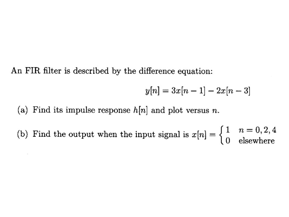
Example: The FIR filter is completely defined once the set of filter coefficients {b k } is known. For example, if the {b k } are then we have a length 4 filter with M = 3. This expands into a 4- point difference equation:

23
To illustrate the utility of the results that we obtained, consider the cascade of two systems defined by: The overall cascade system has the impulse response convolution

24
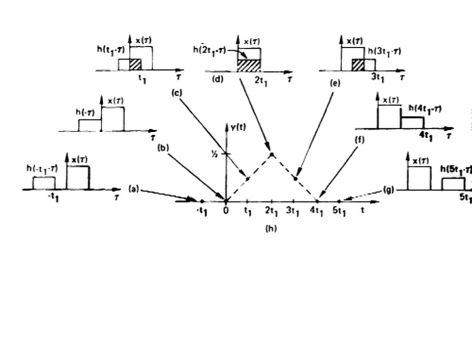
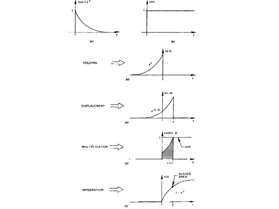
In the analog world, convolution is described by the equation: Constant with respect to . Rotated about the y-axis. Moves along the x-axis.

27
In order to find the overall impulse response we must convolve h 1 [n] with h 2 [n]. Thus, the equivalent impulse response is n0 1 2 3 4 5 h_1[n]1 1 1 1 h_2[n]1 1 1 h_1[0] h_2[n]1 1 1 1 h_1[1] h_2[n] 1 1 1 1 h_1[2] h_2[n] 1 1 1 1 h[n]1 2 3 3 2 1
![In order to find the overall impulse response we must convolve h 1 [n] with h 2 [n].](http://images.slideplayer.com/18/6166400/slides/slide_27.jpg "Thus, the equivalent impulse response is n h_1[n] h_2[n]1 1 1 h_1[0] h_2[n] h_1[1] h_2[n] h_1[2] h_2[n] h[n]")
28
Thus, the equivalent impulse response is where {b k } is the sequence {1, 2, 3, 3, 2, 1}. This means that a system with impulse response h[n] can be implemented by the single difference equation

29
Use convolution to compute the output y[n] for the length 4 filter that have the coefficients b k = {1, -2, 2, -1}. Use the input signal shown below.
![Use convolution to compute the output y[n] for the length 4 filter that have the coefficients b k = {1, -2, 2, -1}.](http://images.slideplayer.com/18/6166400/slides/slide_29.jpg "Use the input signal shown below..")
31
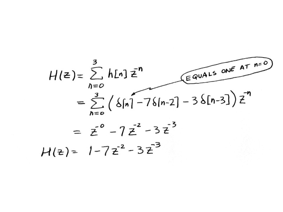
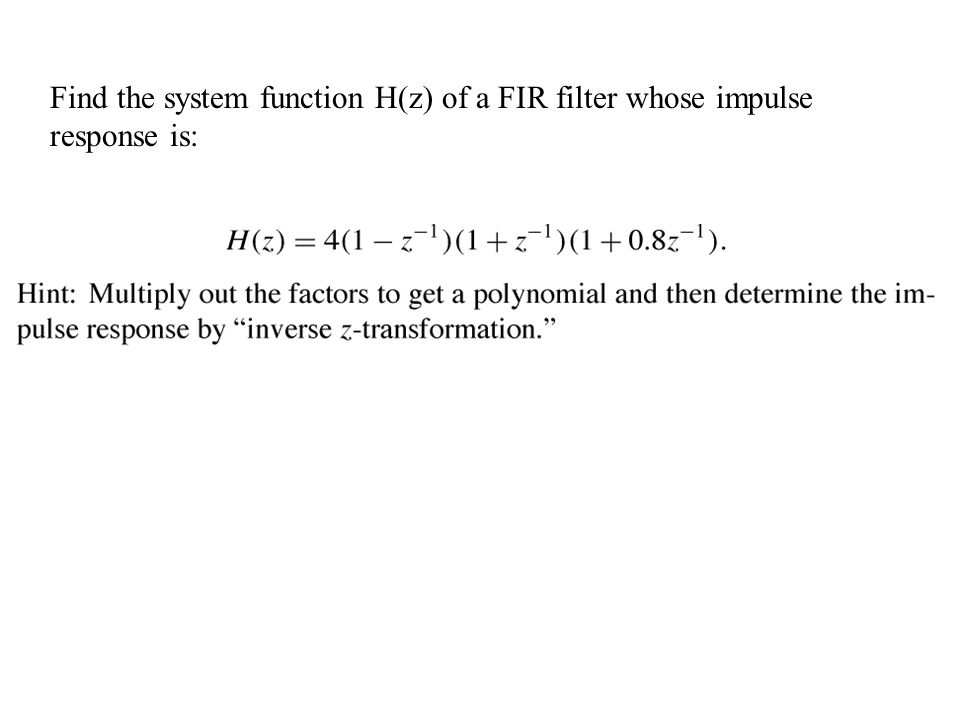
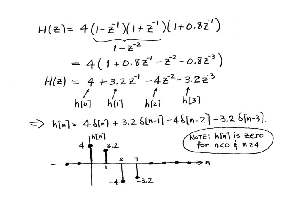
Find the system function H(z) of a FIR filter whose impulse response is:
 of a FIR filter whose impulse response is:")
35
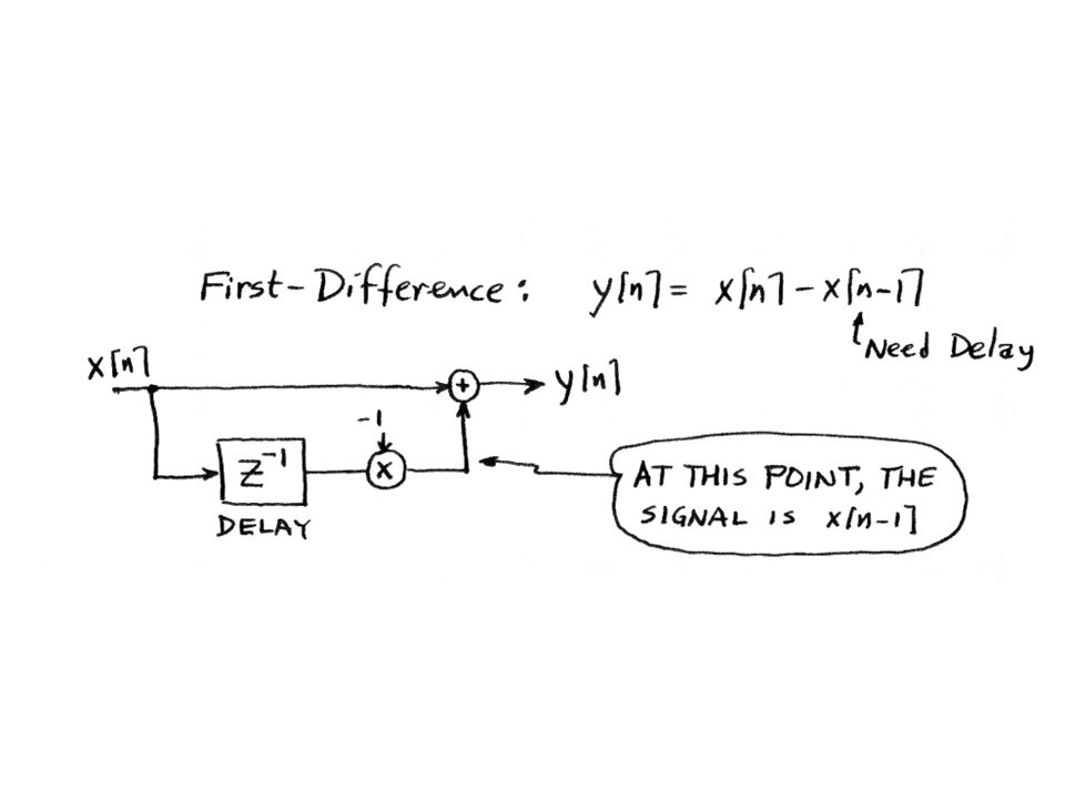
Compuational structure for a first order FIR filter. (a) The equivalence between z -1 and the unit delay; (b) Block diagram for the first order filter whose difference equation is y[n] = b 0 x[n] + b 1 x[n-1]. Draw a block diagram similar to (b) for the first difference system: y[n] = (1- z -1 ){x[n]}.
 The equivalence between z -1 and the unit delay; (b) Block diagram for the first order filter whose difference equation is y[n] = b 0 x[n] + b 1 x[n-1]. Draw a block diagram similar to (b) for the first difference system: y[n] = (1- z -1 ){x[n]}..")
Similar presentations