Download presentation
Presentation is loading. Please wait.

1
Algorithms for Large Sequential Incomplete-Information Games Tuomas Sandholm Professor Carnegie Mellon University Computer Science Department

2
Most real-world games are incomplete-information games with sequential (& simultaneous) moves Negotiation Multi-stage auctions (e.g., FCC ascending, combinatorial auctions) Sequential auctions of multiple items A robot facing adversaries in uncertain, stochastic envt Card games, e.g., poker Currency attacks International (over-)fishing Political campaigns (e.g., TV spending in each region) Ownership games (polar regions, moons, planets) Allocating (and timing) troops/armaments to locations –US allocating troops in Afghanistan & Iraq –Military spending games, e.g., space vs ocean –Airport security, air marshals, coast guard, rail [joint w Tambe] –Cybersecurity...
![Most real-world games are incomplete-information games with sequential (& simultaneous) moves Negotiation Multi-stage auctions (e.g., FCC ascending, combinatorial auctions) Sequential auctions of multiple items A robot facing adversaries in uncertain, stochastic envt Card games, e.g., poker Currency attacks International (over-)fishing Political campaigns (e.g., TV spending in each region) Ownership games (polar regions, moons, planets) Allocating (and timing) troops/armaments to locations –US allocating troops in Afghanistan & Iraq –Military spending games, e.g., space vs ocean –Airport security, air marshals, coast guard, rail [joint w Tambe] –Cybersecurity...](http://images.slideplayer.com/18/6166328/slides/slide_2.jpg "Most real-world games are incomplete-information games with sequential (& simultaneous) moves Negotiation Multi-stage auctions (e.g., FCC ascending, combinatorial auctions) Sequential auctions of multiple items A robot facing adversaries in uncertain, stochastic envt Card games, e.g., poker Currency attacks International (over-)fishing Political campaigns (e.g., TV spending in each region) Ownership games (polar regions, moons, planets) Allocating (and timing) troops/armaments to locations –US allocating troops in Afghanistan & Iraq –Military spending games, e.g., space vs ocean –Airport security, air marshals, coast guard, rail [joint w Tambe] –Cybersecurity...")
3
Sequential incomplete-information games Challenges –Imperfect information –Risk assessment and management –Speculation and counter-speculation: Interpreting signals and avoiding signaling too much Techniques for complete-info games don’t apply Techniques I will discuss are domain-independent

4
Game theory Definition. Strategy is a mapping from known history to action In multi-agent systems, an agent’s outcome depends on the actions of others’ =>Agent’s optimal strategy depends on others’ strategies Definition. A (Bayes) Nash equilibrium is a strategy (and beliefs) for each agent such that no agent benefits from using a different strategy
 Nash equilibrium is a strategy (and beliefs) for each agent such that no agent benefits from using a different strategy.")
5
Simple example Rock Paper Scissors Paper 1/3 Player 1 Player 2 0, 0-1, 11, -1 0, 0-1, 1 1, -10, 0

6
Basics about Nash equilibria In 2-person 0-sum games, –Nash equilibria are minimax equilibria => no equilibrium selection problem –If opponent plays a non-equilibrium strategy, that only helps me Any finite sequential game (satisfying perfect recall) can be converted into a matrix game –Exponential blowup in #strategies Sequence form: More compact representation based on sequences of moves rather than pure strategies [Romanovskii 62, Koller & Megiddo 92, von Stengel 96] –2-person 0-sum games with perfect recall can be solved in time polynomial in size of game tree using LP –Cannot solve Rhode Island Hold’em (3.1 billion nodes) or Texas Hold’em (10 18 nodes)
![Basics about Nash equilibria In 2-person 0-sum games, –Nash equilibria are minimax equilibria => no equilibrium selection problem –If opponent plays a non-equilibrium strategy, that only helps me Any finite sequential game (satisfying perfect recall) can be converted into a matrix game –Exponential blowup in #strategies Sequence form: More compact representation based on sequences of moves rather than pure strategies [Romanovskii 62, Koller & Megiddo 92, von Stengel 96] –2-person 0-sum games with perfect recall can be solved in time polynomial in size of game tree using LP –Cannot solve Rhode Island Hold’em (3.1 billion nodes) or Texas Hold’em (10 18 nodes)](http://images.slideplayer.com/18/6166328/slides/slide_6.jpg "Basics about Nash equilibria In 2-person 0-sum games, –Nash equilibria are minimax equilibria => no equilibrium selection problem –If opponent plays a non-equilibrium strategy, that only helps me Any finite sequential game (satisfying perfect recall) can be converted into a matrix game –Exponential blowup in #strategies Sequence form: More compact representation based on sequences of moves rather than pure strategies [Romanovskii 62, Koller & Megiddo 92, von Stengel 96] –2-person 0-sum games with perfect recall can be solved in time polynomial in size of game tree using LP –Cannot solve Rhode Island Hold’em (3.1 billion nodes) or Texas Hold’em (10 18 nodes)")
7
Extensive form representation Players I = {0, 1, …, n} Tree (V,E) Terminals Z V Controlling player P: V \ Z H Information sets H={H 0,…, H n } Actions A = {A 0, …, A n } Payoffs u : Z R n Chance probabilities p Perfect recall assumption: Players never forget information Game from: Bernhard von Stengel. Efficient Computation of Behavior Strategies. In Games and Economic Behavior 14:220-246, 1996.

8
Computing equilibria via normal form Normal form exponential, in worst case and in practice (e.g. poker)
.")
9
Sequence form [Romanovskii 62, re-invented in English-speaking literature: Koller & Megiddo 92, von Stengel 96] Instead of a move for every information set, consider choices necessary to reach each information set and each leaf These choices are sequences and constitute the pure strategies in the sequence form S 1 = {{}, l, r, L, R} S 2 = {{}, c, d}
![Sequence form [Romanovskii 62, re-invented in English-speaking literature: Koller & Megiddo 92, von Stengel 96] Instead of a move for every information set, consider choices necessary to reach each information set and each leaf These choices are sequences and constitute the pure strategies in the sequence form S 1 = {{}, l, r, L, R} S 2 = {{}, c, d}](http://images.slideplayer.com/18/6166328/slides/slide_9.jpg "Sequence form [Romanovskii 62, re-invented in English-speaking literature: Koller & Megiddo 92, von Stengel 96] Instead of a move for every information set, consider choices necessary to reach each information set and each leaf These choices are sequences and constitute the pure strategies in the sequence form S 1 = {{}, l, r, L, R} S 2 = {{}, c, d}")
10
Realization plans Players’ strategies are specified as realization plans over sequences: Prop. Realization plans are equivalent to behavior strategies.

11
Computing equilibria via sequence form Players 1 and 2 have realization plans x and y Realization constraint matrices E and F specify constraints on realizations {} l r L R {} c d {} v v’ {} u

12
Computing equilibria via sequence form Payoffs for player 1 and 2 are: and for suitable matrices A and B Creating payoff matrix: –Initialize each entry to 0 –For each leaf, there is a (unique) pair of sequences corresponding to an entry in the payoff matrix –Weight the entry by the product of chance probabilities along the path from the root to the leaf {} c d {} l r L R
 pair of sequences corresponding to an entry in the payoff matrix –Weight the entry by the product of chance probabilities along the path from the root to the leaf {} c d {} l r L R")
13
Computing equilibria via sequence form PrimalDual Holding x fixed, compute best response Holding y fixed, compute best response Primal Dual Now, assume 0-sum. The latter primal and dual must have same optimal value e T p. That is the amount that player 2, if he plays y, has to give to player 1, so player 2 tries to minimize it:

14
Computing equilibria via sequence form: An example min p1 subject to x1: p1 - p2 - p3 >= 0 x2: 0y1 + p2 >= 0 x3: -y2 + y3 + p2 >= 0 x4: 2y2 - 4y3 + p3 >= 0 x5: -y1 + p3 >= 0 q1: -y1 = -1 q2: y1 - y2 - y3 = 0 bounds y1 >= 0 y2 >= 0 y3 >= 0 p1 Free p2 Free p3 Free

15
Sequence form summary Polytime algorithm for finding a Nash equilibrium in 2- player zero-sum games Polysize linear complementarity problem (LCP) for computing Nash equilibria in 2-player general-sum games Major shortcomings: –Not well understood when more than two players –Sometimes, polynomial is still slow and or large (e.g. poker)…
….")
16
Games and information Games can be differentiated based on the information available to the players –Perfect information games: players have complete knowledge about the state of the world Examples: Chess, Go, Checkers –Imperfect information games: players face uncertainty about the state of the world Examples: –A robot facing adversaries in an uncertain, stochastic environment –Almost any economic situation in which the other participants possess private information (e.g. valuations, quality information) –Almost any card game in which the other players’ cards are hidden This class of games presents several challenges for AI –Imperfect information –Risk assessment and management –Speculation and counter-speculation
 –Almost any card game in which the other players’ cards are hidden This class of games presents several challenges for AI –Imperfect information –Risk assessment and management –Speculation and counter-speculation.")
17
Poker Recognized challenge problem in AI –Hidden information (other players’ cards) –Uncertainty about future events –Deceptive strategies needed in a good player Very large game trees Texas Hold’em is the most popular variant On NBC:
 –Uncertainty about future events –Deceptive strategies needed in a good player Very large game trees Texas Hold’em is the most popular variant On NBC:")
18
Outline Abstraction Equilibrium finding in 2-person 0-sum games Strategy purification Opponent exploitation Multiplayer stochastic games Leveraging qualitative models

19
Other methods for finding equilibria Fictitious play –Convergence only guaranteed for zero-sum games Tabu best-response search [Sureka & Wurman 2005] –Finds pure strategy equilibria –Does not require game to be completely specified Lemke-Howson algorithm –Pivoting algorithm for finding one Nash equilibrium –Very similar to the simplex algorithm for LP Support enumeration methods –Porter-Nudelman-Shoham [2004] –Mixed-Integer Programming Nash [Sandholm et al 2005]
![Other methods for finding equilibria Fictitious play –Convergence only guaranteed for zero-sum games Tabu best-response search [Sureka & Wurman 2005] –Finds pure strategy equilibria –Does not require game to be completely specified Lemke-Howson algorithm –Pivoting algorithm for finding one Nash equilibrium –Very similar to the simplex algorithm for LP Support enumeration methods –Porter-Nudelman-Shoham [2004] –Mixed-Integer Programming Nash [Sandholm et al 2005]](http://images.slideplayer.com/18/6166328/slides/slide_19.jpg "Other methods for finding equilibria Fictitious play –Convergence only guaranteed for zero-sum games Tabu best-response search [Sureka & Wurman 2005] –Finds pure strategy equilibria –Does not require game to be completely specified Lemke-Howson algorithm –Pivoting algorithm for finding one Nash equilibrium –Very similar to the simplex algorithm for LP Support enumeration methods –Porter-Nudelman-Shoham [2004] –Mixed-Integer Programming Nash [Sandholm et al 2005]")
20
Our approach Automated abstraction + equilibrium finding

21
Our approach [Gilpin & S., EC’06, JACM’07…] Now used by all competitive Texas Hold’em programs Nash equilibrium Original game Abstracted game Automated abstraction Custom equilibrium-finding algorithm Reverse model
![Our approach [Gilpin & S., EC’06, JACM’07…] Now used by all competitive Texas Hold’em programs Nash equilibrium Original game Abstracted game Automated abstraction Custom equilibrium-finding algorithm Reverse model](http://images.slideplayer.com/18/6166328/slides/slide_21.jpg "Our approach [Gilpin & S., EC’06, JACM’07…] Now used by all competitive Texas Hold’em programs Nash equilibrium Original game Abstracted game Automated abstraction Custom equilibrium-finding algorithm Reverse model")
22
Outline Automated abstraction –Lossless –Lossy New equilibrium-finding algorithms

23
Outline Automated abstraction –Lossless –Lossy New equilibrium-finding algorithms Stochastic games with >2 players, e.g., poker tournaments Current & future research

24
Outline Lossless automated abstraction –Optimal strategies for Rhode Island Hold’em Approximate automated abstraction –“Greedy” (GS1) –Clustering and integer programming (GS2) –Potential-aware (GS3) Equilibrium-finding algorithms –Adapting Nesterov’s excessive gap technique to sequential games –Making it scalable –New related algorithm with exponentially better speed Future research Thoughts on application games of national importance
 –Clustering and integer programming (GS2) –Potential-aware (GS3) Equilibrium-finding algorithms –Adapting Nesterov’s excessive gap technique to sequential games –Making it scalable –New related algorithm with exponentially better speed Future research Thoughts on application games of national importance")
25
Our approach We introduce automated abstraction techniques that result in smaller, (nearly) equivalent games –For the optimal version of our algorithm: We prove that a Nash equilibrium in the smaller game corresponds to a Nash equilibrium in the original game The smaller game can then be solved using standard techniques –For the approximate versions of our algorithm: We demonstrate their effectiveness by applying the algorithm to Texas Hold’em poker and comparing with other poker-playing programs We also improve the equilibrium-finding algorithms themselves
 equivalent games –For the optimal version of our algorithm: We prove that a Nash equilibrium in the smaller game corresponds to a Nash equilibrium in the original game The smaller game can then be solved using standard techniques –For the approximate versions of our algorithm: We demonstrate their effectiveness by applying the algorithm to Texas Hold’em poker and comparing with other poker-playing programs We also improve the equilibrium-finding algorithms themselves")
26
Game with ordered signals (a.k.a. ordered game) 1.Players I = {1,…,n} 2.Stage games G = G 1,…,G r 3.Player label L 4.Game-ending nodes ω 5.Signal alphabet Θ 6.Signal quantities κ = κ 1,…,κ r and γ = γ 1,…,γ r 7.Signal probability distribution p 8.Partial ordering ≥ of subsets of Θ 9.Utility function u (increasing in private signals) I = {1,2} Θ = {2♠,…,A♦} κ = (0,1,1) γ = (1,0,0) UniformHand rank
 1.Players I = {1,…,n} 2.Stage games G = G 1,…,G r 3.Player label L 4.Game-ending nodes ω 5.Signal alphabet Θ 6.Signal quantities κ = κ 1,…,κ r and γ = γ 1,…,γ r 7.Signal probability distribution p 8.Partial ordering ≥ of subsets of Θ 9.Utility function u (increasing in private signals) I = {1,2} Θ = {2♠,…,A♦} κ = (0,1,1) γ = (1,0,0) UniformHand rank.")
27
Reasons to abstract Scalability (computation speed & memory) Game may be so complicated that can’t model without abstraction Existence of equilibrium, or solving algorithm, may require a certain kind of game, e.g., finite
 Game may be so complicated that can’t model without abstraction Existence of equilibrium, or solving algorithm, may require a certain kind of game, e.g., finite")
28
Lossless abstraction [Gilpin & S., EC’06, JACM’07]
![Lossless abstraction [Gilpin & S., EC’06, JACM’07]](http://images.slideplayer.com/18/6166328/slides/slide_28.jpg "Lossless abstraction [Gilpin & S., EC’06, JACM’07]")
29
Information filters Observation: We can make games smaller by filtering the information a player receives Instead of observing a specific signal exactly, a player instead observes a filtered set of signals –E.g. receiving signal {A♠,A♣,A♥,A♦} instead of A♥

30
Signal tree Each edge corresponds to the revelation of some signal by nature to at least one player Our lossless abstraction algorithm operates on it –Don’t load full game into memory

31
Isomorphic relation Captures the notion of strategic symmetry between nodes Defined recursively: –Two leaves in signal tree are isomorphic if for each action history in the game, the payoff vectors (one payoff per player) are the same –Two internal nodes in signal tree are isomorphic if they are siblings and there is a bijection between their children such that only ordered game isomorphic nodes are matched We compute this relationship for all nodes using a DP plus custom perfect matching in a bipartite graph
 are the same –Two internal nodes in signal tree are isomorphic if they are siblings and there is a bijection between their children such that only ordered game isomorphic nodes are matched We compute this relationship for all nodes using a DP plus custom perfect matching in a bipartite graph")
32
Abstraction transformation Merges two isomorphic nodes Theorem. If a strategy profile is a Nash equilibrium in the abstracted (smaller) game, then its interpretation in the original game is a Nash equilibrium Assumptions –Observable player actions –Players’ utility functions rank the signals in the same order
 game, then its interpretation in the original game is a Nash equilibrium Assumptions –Observable player actions –Players’ utility functions rank the signals in the same order.")
36
GameShrink algorithm Bottom-up pass: Run DP to mark isomorphic pairs of nodes in signal tree Top-down pass: Starting from top of signal tree, perform the transformation where applicable Theorem. Conducts all these transformations –Õ(n 2 ), where n is #nodes in signal tree –Usually highly sublinear in game tree size
, where n is #nodes in signal tree –Usually highly sublinear in game tree size.")
37
Algorithmic techniques for making GameShrink faster Union-Find data structure for efficient representation of the information filter (unioning finer signals into coarser signals) –Linear memory and almost linear time Eliminate some perfect matching computations using easy-to-check necessary conditions –Compact histogram databases for storing win/loss frequencies to speed up the checks
 –Linear memory and almost linear time Eliminate some perfect matching computations using easy-to-check necessary conditions –Compact histogram databases for storing win/loss frequencies to speed up the checks")
38
Solved Rhode Island Hold’em poker AI challenge problem [Shi & Littman 01] –3.1 billion nodes in game tree Without abstraction, LP has 91,224,226 rows and columns => unsolvable GameShrink runs in one second After that, LP has 1,237,238 rows and columns Solved the LP –CPLEX barrier method took 8 days & 25 GB RAM Exact Nash equilibrium Largest incomplete-info game solved by then by over 4 orders of magnitude
![Solved Rhode Island Hold’em poker AI challenge problem [Shi & Littman 01] –3.1 billion nodes in game tree Without abstraction, LP has 91,224,226 rows and columns => unsolvable GameShrink runs in one second After that, LP has 1,237,238 rows and columns Solved the LP –CPLEX barrier method took 8 days & 25 GB RAM Exact Nash equilibrium Largest incomplete-info game solved by then by over 4 orders of magnitude](http://images.slideplayer.com/18/6166328/slides/slide_38.jpg "Solved Rhode Island Hold’em poker AI challenge problem [Shi & Littman 01] –3.1 billion nodes in game tree Without abstraction, LP has 91,224,226 rows and columns => unsolvable GameShrink runs in one second After that, LP has 1,237,238 rows and columns Solved the LP –CPLEX barrier method took 8 days & 25 GB RAM Exact Nash equilibrium Largest incomplete-info game solved by then by over 4 orders of magnitude")
39
Lossy abstraction

40
Prior game abstractions (automated or manual) Lossless [Gilpin & Sandholm, EC’06, JACM’07] Lossy without bound [Shi and Littman CG-02; Billings et al. IJCAI-03; Gilpin & Sandholm, AAAI-06, -08, AAMAS-07; Gilpin, Sandholm & Soerensen AAAI-07, AAMAS-08; Zinkevich et al. NIPS-07; Waugh et al. AAMAS-09, SARA-09;…] –Exploitability can sometimes be checked ex post [Johanson et al. IJCAI-11]
![Prior game abstractions (automated or manual) Lossless [Gilpin & Sandholm, EC’06, JACM’07] Lossy without bound [Shi and Littman CG-02; Billings et al.](http://images.slideplayer.com/18/6166328/slides/slide_40.jpg "IJCAI-03; Gilpin & Sandholm, AAAI-06, -08, AAMAS-07; Gilpin, Sandholm & Soerensen AAAI-07, AAMAS-08; Zinkevich et al. NIPS-07; Waugh et al. AAMAS-09, SARA-09;…] –Exploitability can sometimes be checked ex post [Johanson et al. IJCAI-11].")
41
We developed many lossy abstraction algorithms Scalable to large n-player, general-sum games, e.g., Texas Hold’em Gilpin, A. and Sandholm, T. 2008. Expectation-Based Versus Potential- Aware Automated Abstraction in Imperfect Information Games: An Experimental Comparison Using Poker. AAAI.Expectation-Based Versus Potential- Aware Automated Abstraction in Imperfect Information Games: An Experimental Comparison Using Poker. Gilpin, A., Sandholm, T., Troels Bjerre Sørensen 2008. A heads-up no-limit Texas Hold'em poker player: Discretized betting models and automatically generated equilibrium-finding programs. AAMAS.A heads-up no-limit Texas Hold'em poker player: Discretized betting models and automatically generated equilibrium-finding programs. Gilpin, A., Sandholm, T., Soerensen, T. 2007. Potential-Aware Automated Abstraction of Sequential Games, and Holistic Equilibrium Analysis of Texas Hold'em Poker. AAAI.Potential-Aware Automated Abstraction of Sequential Games, and Holistic Equilibrium Analysis of Texas Hold'em Poker. Gilpin, A., Sandholm, T. 2007. Better automated abstraction techniques for imperfect information games, with application to Texas Hold'em poker. In AAMAS.Better automated abstraction techniques for imperfect information games, with application to Texas Hold'em poker. Gilpin, A., Sandholm, T. 2006. A competitive Texas Hold'em Poker player via automated abstraction and real-time equilibrium computation. AAAI.A competitive Texas Hold'em Poker player via automated abstraction and real-time equilibrium computation.

42
Texas Hold’em poker

51
2-player Limit Texas Hold’em has ~10 18 leaves in game tree Losslessly abstracted game too big to solve => abstract more => lossy Nature deals 2 cards to each player Nature deals 3 shared cards Nature deals 1 shared card Round of betting

52
GS1 [Gilpin & S., AAAI’06] First Texas Hold’em program to use automated abstraction –Lossy version of Gameshrink Instead of requiring perfect matching of children, require a matching with a penalty below threshold Abstracted game’s LP solved by CPLEX Phase I (rounds 1 & 2) LP solved offline –Assuming rollout for the rest of the game Phase II (rounds 3 & 4) LP solved in real time –Starting with hand probabilities that are updated using Bayes rule based on Phase I equilibrium and observations
![GS1 [Gilpin & S., AAAI’06] First Texas Hold’em program to use automated abstraction –Lossy version of Gameshrink Instead of requiring perfect matching of children, require a matching with a penalty below threshold Abstracted game’s LP solved by CPLEX Phase I (rounds 1 & 2) LP solved offline –Assuming rollout for the rest of the game Phase II (rounds 3 & 4) LP solved in real time –Starting with hand probabilities that are updated using Bayes rule based on Phase I equilibrium and observations](http://images.slideplayer.com/18/6166328/slides/slide_52.jpg "GS1 [Gilpin & S., AAAI’06] First Texas Hold’em program to use automated abstraction –Lossy version of Gameshrink Instead of requiring perfect matching of children, require a matching with a penalty below threshold Abstracted game’s LP solved by CPLEX Phase I (rounds 1 & 2) LP solved offline –Assuming rollout for the rest of the game Phase II (rounds 3 & 4) LP solved in real time –Starting with hand probabilities that are updated using Bayes rule based on Phase I equilibrium and observations")
53
GS1 1/2005 - 1/2006

54
GS1 We split the 4 betting rounds into two phases –Phase I (first 2 rounds) solved offline using approximate version of GameShrink followed by LP Assuming rollout –Phase II (last 2 rounds): abstractions computed offline –betting history doesn’t matter & suit isomorphisms real-time equilibrium computation using anytime LP –updated hand probabilities from Phase I equilibrium (using betting histories and community card history): –s i is player i’s strategy, h is an information set
 solved offline using approximate version of GameShrink followed by LP Assuming rollout –Phase II (last 2 rounds): abstractions computed offline –betting history doesn’t matter & suit isomorphisms real-time equilibrium computation using anytime LP –updated hand probabilities from Phase I equilibrium (using betting histories and community card history): –s i is player i’s strategy, h is an information set")
55
Some additional techniques used Precompute several databases Conditional choice of primal vs. dual simplex for real-time equilibrium computation –Achieve anytime capability for the player that is us Dealing with running off the equilibrium path

56
GS1 results Sparbot: Game-theory-based player, manual abstraction Vexbot: Opponent modeling, miximax search with statistical sampling GS1 performs well, despite using very little domain-knowledge and no adaptive techniques –No statistical significance

57
GS2 [Gilpin & S., AAMAS’07] Original GameShrink is “greedy” when used as an approximation algorithm => lopsided abstractions GS2 instead finds abstraction via clustering & IP –Round by round starting from round 1 –Operates in signal tree of one player’s & common signals at a time Other ideas in GS2: – Overlapping phases so Phase I would be less myopic Phase I = round 1, 2, and 3; Phase II = rounds 3 and 4 –Instead of assuming rollout at leaves of Phase I (as was done in SparBot and GS1), use statistics to get a more accurate estimate of how play will go
![GS2 [Gilpin & S., AAMAS’07] Original GameShrink is greedy when used as an approximation algorithm => lopsided abstractions GS2 instead finds abstraction via clustering & IP –Round by round starting from round 1 –Operates in signal tree of one player’s & common signals at a time Other ideas in GS2: – Overlapping phases so Phase I would be less myopic Phase I = round 1, 2, and 3; Phase II = rounds 3 and 4 –Instead of assuming rollout at leaves of Phase I (as was done in SparBot and GS1), use statistics to get a more accurate estimate of how play will go](http://images.slideplayer.com/18/6166328/slides/slide_57.jpg "GS2 [Gilpin & S., AAMAS’07] Original GameShrink is greedy when used as an approximation algorithm => lopsided abstractions GS2 instead finds abstraction via clustering & IP –Round by round starting from round 1 –Operates in signal tree of one player’s & common signals at a time Other ideas in GS2: – Overlapping phases so Phase I would be less myopic Phase I = round 1, 2, and 3; Phase II = rounds 3 and 4 –Instead of assuming rollout at leaves of Phase I (as was done in SparBot and GS1), use statistics to get a more accurate estimate of how play will go")
58
GS2 2/2006 – 7/2006 [Gilpin & S., AAMAS’07]
![GS2 2/2006 – 7/2006 [Gilpin & S., AAMAS’07]](http://images.slideplayer.com/18/6166328/slides/slide_58.jpg "GS2 2/2006 – 7/2006 [Gilpin & S., AAMAS’07]")
59
Optimized approximate abstractions Original version of GameShrink is “greedy” when used as an approximation algorithm => lopsided abstractions GS2 instead finds an abstraction via clustering & IP For round 1 in signal tree, use 1D k-means clustering –Similarity metric is win probability (ties count as half a win) For each round 2..3 of signal tree: –For each group i of hands (children of a parent at round – 1): use 1D k-means clustering to split group i into k i abstract “states” for each value of k i, compute expected error (considering hand probs) –IP decides how many children different parents (from round – 1) may have: Decide k i ’s to minimize total expected error, subject to ∑ i k i ≤ K round K round is set based on acceptable size of abstracted game Solving this IP is fast in practice
 For each round 2..3 of signal tree: –For each group i of hands (children of a parent at round – 1): use 1D k-means clustering to split group i into k i abstract states for each value of k i, compute expected error (considering hand probs) –IP decides how many children different parents (from round – 1) may have: Decide k i ’s to minimize total expected error, subject to ∑ i k i ≤ K round K round is set based on acceptable size of abstracted game Solving this IP is fast in practice")
60
Phase I (first three rounds) Allowed 15, 225, and 900 abstracted states in rounds 1, 2, and 3, respectively Optimizing the approximate abstraction took 3 days on 4 CPUs LP took 7 days and 80 GB using CPLEX’s barrier method
 Allowed 15, 225, and 900 abstracted states in rounds 1, 2, and 3, respectively Optimizing the approximate abstraction took 3 days on 4 CPUs LP took 7 days and 80 GB using CPLEX’s barrier method")
61
Phase I (first three rounds) Optimized abstraction –Round 1 There are 1,326 hands, of which 169 are strategically different We allowed 15 abstract states –Round 2 There are 25,989,600 distinct possible hands –GameShrink (in lossless mode for Phase I) determined there are ~10 6 strategically different hands Allowed 225 abstract states –Round 3 There are 1,221,511,200 distinct possible hands Allowed 900 abstract states Optimizing the approximate abstraction took 3 days on 4 CPUs LP took 7 days and 80 GB using CPLEX’s barrier method
 Optimized abstraction –Round 1 There are 1,326 hands, of which 169 are strategically different We allowed 15 abstract states –Round 2 There are 25,989,600 distinct possible hands –GameShrink (in lossless mode for Phase I) determined there are ~10 6 strategically different hands Allowed 225 abstract states –Round 3 There are 1,221,511,200 distinct possible hands Allowed 900 abstract states Optimizing the approximate abstraction took 3 days on 4 CPUs LP took 7 days and 80 GB using CPLEX’s barrier method")
62
Mitigating effect of round-based abstraction (i.e., having 2 phases) For leaves of Phase I, GS1 & SparBot assumed rollout Can do better by estimating the actions from later in the game (betting) using statistics For each possible hand strength and in each possible betting situation, we stored the probability of each possible action –Mine history of how betting has gone in later rounds from 100,000’s of hands that SparBot played –E.g. of betting in 4 th round Player 1 has bet. Player 2’s turn

63
Example of betting in 4th round Player 1 has bet. Player 2 to fold, call, or raise

64
Phase II (rounds 3 and 4) Abstraction computed using the same optimized abstraction algorithm as in Phase I Equilibrium solved in real time (as in GS1) –Beliefs for the beginning of Phase II determined using Bayes rule based on observations and the computed equilibrium strategies from Phase I
 Abstraction computed using the same optimized abstraction algorithm as in Phase I Equilibrium solved in real time (as in GS1) –Beliefs for the beginning of Phase II determined using Bayes rule based on observations and the computed equilibrium strategies from Phase I")
65
Precompute several databases db5 : possible wins and losses (for a single player) for every combination of two hole cards and three community cards (25,989,600 entries) –Used by GameShrink for quickly comparing the similarity of two hands db223 : possible wins and losses (for both players) for every combination of pairs of two hole cards and three community cards based on a roll-out of the remaining cards (14,047,378,800 entries) –Used for computing payoffs of the Phase I game to speed up the LP creation handval : concise encoding of a 7-card hand rank used for fast comparisons of hands (133,784,560 entries) –Used in several places, including in the construction of db5 and db223 Colexicographical ordering used to compute indices into the databases allowing for very fast lookups
 for every combination of two hole cards and three community cards (25,989,600 entries) –Used by GameShrink for quickly comparing the similarity of two hands db223 : possible wins and losses (for both players) for every combination of pairs of two hole cards and three community cards based on a roll-out of the remaining cards (14,047,378,800 entries) –Used for computing payoffs of the Phase I game to speed up the LP creation handval : concise encoding of a 7-card hand rank used for fast comparisons of hands (133,784,560 entries) –Used in several places, including in the construction of db5 and db223 Colexicographical ordering used to compute indices into the databases allowing for very fast lookups")
66
GS2 experiments OpponentSeries won by GS2 Win rate (small bets per hand) GS138 of 50 p=.00031 +0.031 Sparbot28 of 50 p=.48 +0.0043 Vexbot32 of 50 p=.065 -0.0062
 GS138 of 50 p= Sparbot28 of 50 p= Vexbot32 of 50 p=")
67
GS3 8/2006 – 3/2007 ø [Gilpin, S. & Sørensen AAAI’07] Our poker bots 2008-2011 were generated with same abstraction algorithm

68
Entire game solved holistically We no longer break game into phases –Because our new equilibrium-finding algorithms can solve games of the size that stem from reasonably fine-grained abstractions of the entire game => better strategies & real-time end-game computation optional

69
Clustering + integer programming for abstraction [Gilpin & Sandholm AAMAS’07] GameShrink is “greedy” when used as an approximation algorithm => lopsided abstractions For constructing GS2, abstraction was created via clustering & IP Operates in signal tree of one player’s & common signals at a time
![Clustering + integer programming for abstraction [Gilpin & Sandholm AAMAS’07] GameShrink is greedy when used as an approximation algorithm => lopsided abstractions For constructing GS2, abstraction was created via clustering & IP Operates in signal tree of one player’s & common signals at a time](http://images.slideplayer.com/18/6166328/slides/slide_69.jpg "Clustering + integer programming for abstraction [Gilpin & Sandholm AAMAS’07] GameShrink is greedy when used as an approximation algorithm => lopsided abstractions For constructing GS2, abstraction was created via clustering & IP Operates in signal tree of one player’s & common signals at a time")
70
ø Potential-aware automated abstraction [Gilpin, S. & Sørensen AAAI’07] All prior abstraction algorithms had EV (myopic probability of winning in poker) as the similarity metric –Doesn’t capture potential Potential not only positive or negative, but also “multidimensional” GS3’s abstraction algorithm captures potential …
 as the similarity metric –Doesn’t capture potential Potential not only positive or negative, but also multidimensional GS3’s abstraction algorithm captures potential ….")
71
Idea: similarity metric between hands at round R should be based on the vector of probabilities of transitions to abstracted states at round R+1 –E.g., L 1 norm In the last round, the similarity metric is simply probability of winning (assuming rollout) This enables a bottom
 This enables a bottom")
72
Bottom-up pass to determine abstraction for round 1 Clustering using L 1 norm –Predetermined number of clusters, depending on size of abstraction we are shooting for In the last (4th) round, there is no more potential => we use probability of winning (e.g., assuming rollout) as similarity metric Round r Round r-1.3.2 0.5
 round, there is no more potential => we use probability of winning (e.g., assuming rollout) as similarity metric Round r Round r")
73
Determining abstraction for round 2 For each 1 st -round bucket i: –Make a bottom-up pass to determine 3 rd -round buckets, considering only hands compatible with i –For k i {1, 2, …, max} Cluster the 2 nd -round hands into k i clusters –based on each hand’s histogram over 3 rd -round buckets IP to decide how many children each 1 st -round bucket may have, subject to ∑ i k i ≤ K 2 –Error metric for each bucket is the sum of L 2 distances of the hands from the bucket’s centroid –Total error to minimize is the sum of the buckets’ errors weighted by the probability of reaching the bucket

74
Determining abstraction for round 3 Done analogously to how we did round 2

75
Determining abstraction for round 4 Done analogously, except that now there is no potential left, so clustering is done based on probability of winning Now we have finished the abstraction!

76
Potential-aware vs win-probability-based abstraction Both use clustering and IP Experiment on Rhode Island Hold’em => Abstracted game solved exactly 13 buckets in first round is lossless Potential-aware becomes lossless, win-probability-based is as good as it gets, never lossless Finer-grained abstraction [Gilpin & S., AAAI-08]
![Potential-aware vs win-probability-based abstraction Both use clustering and IP Experiment on Rhode Island Hold’em => Abstracted game solved exactly 13 buckets in first round is lossless Potential-aware becomes lossless, win-probability-based is as good as it gets, never lossless Finer-grained abstraction [Gilpin & S., AAAI-08]](http://images.slideplayer.com/18/6166328/slides/slide_76.jpg "Potential-aware vs win-probability-based abstraction Both use clustering and IP Experiment on Rhode Island Hold’em => Abstracted game solved exactly 13 buckets in first round is lossless Potential-aware becomes lossless, win-probability-based is as good as it gets, never lossless Finer-grained abstraction [Gilpin & S., AAAI-08]")
77
Potential-aware vs win-probability-based abstraction Both use clustering and IP Experiment conducted on Heads-Up Rhode Island Hold’em –Abstracted game solved exactly 13 buckets in first round is lossless Potential-aware becomes lossless, win-probability-based is as good as it gets, never lossless [Gilpin & S., AAAI-08 & new]
![Potential-aware vs win-probability-based abstraction Both use clustering and IP Experiment conducted on Heads-Up Rhode Island Hold’em –Abstracted game solved exactly 13 buckets in first round is lossless Potential-aware becomes lossless, win-probability-based is as good as it gets, never lossless [Gilpin & S., AAAI-08 & new]](http://images.slideplayer.com/18/6166328/slides/slide_77.jpg "Potential-aware vs win-probability-based abstraction Both use clustering and IP Experiment conducted on Heads-Up Rhode Island Hold’em –Abstracted game solved exactly 13 buckets in first round is lossless Potential-aware becomes lossless, win-probability-based is as good as it gets, never lossless [Gilpin & S., AAAI-08 & new]")
78
Other forms of lossy abstraction Phase-based abstraction –Uses observations and equilibrium strategies to infer priors for next phase –Uses some (good) fixed strategies to estimate leaf payouts at non-last phases [Gilpin & Sandholm AAMAS-07] –Supports real-time equilibrium finding [Gilpin & Sandholm AAMAS-07] Grafting [Waugh et al. 2009] as an extension Action abstraction –What if opponents play outside the abstraction? –Multiplicative action similarity and probabilistic reverse model [Gilpin, Sandholm, & Sørensen AAMAS-08, Risk & Szafron AAMAS-10]
![Other forms of lossy abstraction Phase-based abstraction –Uses observations and equilibrium strategies to infer priors for next phase –Uses some (good) fixed strategies to estimate leaf payouts at non-last phases [Gilpin & Sandholm AAMAS-07] –Supports real-time equilibrium finding [Gilpin & Sandholm AAMAS-07] Grafting [Waugh et al.](http://images.slideplayer.com/18/6166328/slides/slide_78.jpg "2009] as an extension Action abstraction –What if opponents play outside the abstraction. –Multiplicative action similarity and probabilistic reverse model [Gilpin, Sandholm, & Sørensen AAMAS-08, Risk & Szafron AAMAS-10].")
79
Game abstraction is nonmonotonic Such “abstraction pathologies” also in small poker games [Waugh et al. AAMAS-09] We present the first lossy game abstraction algorithm with bounds –Contradiction? 0, 21, 12, 0 1, 10, 2 Attacker Defender A A B B Between In each equilibrium: Attacker randomizes 50-50 between A and B Defender plays A w.p. p, B w.p. p, and Between w.p. 1-2p There is an equilibrium for each p [0, ½] 0, 21, 12, 0 A A B Between An abstraction: Defender would choose A, but that is far from equilibrium in the original game where attacker would choose B 1, 12, 0 A B Between Coarser abstraction: Defender would choose Between. That is an equilibrium in the original game

80
First lossy game abstraction algorithms with bounds [Sandholm and Singh EC-12] Recognized open problem; tricky due to pathologies For both action and state abstraction; for finite stochastic games Evaluations from abstract game are near accurate: Regret is bounded:
![First lossy game abstraction algorithms with bounds [Sandholm and Singh EC-12] Recognized open problem; tricky due to pathologies For both action and state abstraction; for finite stochastic games Evaluations from abstract game are near accurate: Regret is bounded:](http://images.slideplayer.com/18/6166328/slides/slide_80.jpg "First lossy game abstraction algorithms with bounds [Sandholm and Singh EC-12] Recognized open problem; tricky due to pathologies For both action and state abstraction; for finite stochastic games Evaluations from abstract game are near accurate: Regret is bounded:")
81
First lossy game abstraction methods with bounds [Sandholm and Singh EC-12] Recognized open problem; tricky due to pathologies For both action and state abstraction For stochastic games
![First lossy game abstraction methods with bounds [Sandholm and Singh EC-12] Recognized open problem; tricky due to pathologies For both action and state abstraction For stochastic games](http://images.slideplayer.com/18/6166328/slides/slide_81.jpg "First lossy game abstraction methods with bounds [Sandholm and Singh EC-12] Recognized open problem; tricky due to pathologies For both action and state abstraction For stochastic games")
82
Strategy evaluation in M and M’ LEMMA. If game M and abstraction M’ are “close”, then the value for every strategy in M’ (when evaluated in M’) is close to the value of any corresponding lifted strategy in M when evaluated in M. Formally: joint strategy
 is close to the value of any corresponding lifted strategy in M when evaluated in M. Formally: joint strategy.")
83
Main abstraction theorem Given a subgame perfect Nash equilibrium in M’ Let lifted strategy in M be Then maximum gain by unilateral deviation by agent i is

84
First lossy game abstraction algorithms with bounds Greedy algorithm that proceeds level by level from end of game –At each level, does either action or state abstraction first, then the other –Polynomial time (versus equilibrium finding being PPAD-complete) Integer linear program –Proceeds level by level from end of game; one ILP per level Optimizing all levels simultaneously would be nonlinear –Does action and state abstraction simultaneously –Splits the allowed total error within level optimally between reward error and transition probability error, and between action abstraction and state abstraction Proposition. Both algorithms satisfy the given bounds on regret Proposition. Even with just action abstraction and just one level, finding the abstraction with the smallest number of actions that respects the regret bound is NP-complete (even with 2 agents) One of the first action abstraction algorithms –Totally different than the prior one [Hawkin et al. AAAI-11]
 One of the first action abstraction algorithms –Totally different than the prior one [Hawkin et al. AAAI-11].")
85
Role of this in modeling All modeling is abstraction! These are the first results that tie game modeling choices to solution quality in the actual setting

86
Strategy-based abstraction [unpublished] Abstraction Equilibrium finding
![Strategy-based abstraction [unpublished] Abstraction Equilibrium finding](http://images.slideplayer.com/18/6166328/slides/slide_86.jpg "Strategy-based abstraction [unpublished] Abstraction Equilibrium finding")
87
Equilibrium-finding algorithms Solving the (abstracted) game
 game")
88
Outline Abstraction Equilibrium finding in 2-person 0-sum games Strategy purification Opponent exploitation Multiplayer stochastic games Leveraging qualitative models

89
Scalability of (near-)equilibrium finding in 2-person 0-sum games Manual approaches can only solve games with a handful of nodes AAAI poker competition announced Koller & Pfeffer Using sequence form & LP (simplex) Billings et al. LP (CPLEX interior point method) Gilpin & Sandholm LP (CPLEX interior point method) Gilpin, Hoda, Peña & Sandholm Scalable EGT Gilpin, Sandholm ø & Sørensen Scalable EGT Zinkevich et al. Counterfactual regret
 Gilpin & Sandholm LP (CPLEX interior point method) Gilpin, Hoda, Peña & Sandholm Scalable EGT Gilpin, Sandholm ø & Sørensen Scalable EGT Zinkevich et al. Counterfactual regret.")
90
(Un)scalability of LP solvers Rhode Island Hold’em LP –91,000,000 rows and columns –After GameShrink,1,200,000 rows and columns, and 50,000,000 non-zeros –CPLEX’s barrier method uses 25 GB RAM and 8 days Texas Hold’em poker much larger –=> would need to use extremely coarse abstraction Instead of LP, can we solve the equilibrium-finding problem in some other way?
scalability of LP solvers Rhode Island Hold’em LP –91,000,000 rows and columns –After GameShrink,1,200,000 rows and columns, and 50,000,000 non-zeros –CPLEX’s barrier method uses 25 GB RAM and 8 days Texas Hold’em poker much larger –=> would need to use extremely coarse abstraction Instead of LP, can we solve the equilibrium-finding problem in some other way")
91
Excessive gap technique (EGT) Best general LP solvers only scale to10 7..10 8 nodes. Can we do better? Usually, gradient-based algorithms have poor O(1/ ε 2 ) convergence, but… Theorem [Nesterov 05]. Gradient-based algorithm, EGT (for a class of minmax problems) that finds an ε-equilibrium in O(1/ ε) iterations Theorem [Hoda, Gilpin, Pena & S., Mathematics of Operations Research 2010]. Nice prox functions can be constructed for sequential games
 convergence, but… Theorem [Nesterov 05]. Gradient-based algorithm, EGT (for a class of minmax problems) that finds an ε-equilibrium in O(1/ ε) iterations Theorem [Hoda, Gilpin, Pena & S., Mathematics of Operations Research 2010]. Nice prox functions can be constructed for sequential games.")
92
Scalable EGT [Gilpin, Hoda, Peña, S., WINE’07, Math. Of OR 2010] Memory saving in poker & many other games Main space bottleneck is storing the game’s payoff matrix A Definition. Kronecker product In Rhode Island Hold’em: Using independence of card deals and betting options, can represent this as A 1 = F 1 B 1 A 2 = F 2 B 2 A 3 = F 3 B 3 + S W F r corresponds to sequences of moves in round r that end in a fold S corresponds to sequences of moves in round 3 that end in a showdown B r encodes card buckets in round r W encodes win/loss/draw probabilities of the buckets

93
Memory usage InstanceCPLEX barrier CPLEX simplex Our method Losslessly abstracted Rhode Island Hold’em 25.2 GB>3.45 GB0.15 GB Lossily abstracted Texas Hold’em >458 GB 2.49 GB

94
Memory usage InstanceCPLEX barrier CPLEX simplex Our method 10k0.082 GB>0.051 GB0.012 GB 160k2.25 GB>0.664 GB0.035 GB Losslessly abstracted RI Hold’em 25.2 GB>3.45 GB0.15 GB Lossily abstracted TX Hold’em >458 GB 2.49 GB

95
Scalable EGT [Gilpin, Hoda, Peña, S., WINE’07, Math. Of OR 2010] Speed Fewer iterations –With Euclidean prox fn, gap was reduced by an order of magnitude more (at given time allocation) compared to entropy-based prox fn –Heuristics that speed things up in practice while preserving theoretical guarantees Less conservative shrinking of 1 and 2 – Sometimes need to reduce (halve) Balancing 1 and 2 periodically –Often allows reduction in the values Gap was reduced by an order of magnitude (for given time allocation) Faster iterations –Parallelization in each of the 3 matrix-vector products in each iteration => near-linear speedup
 compared to entropy-based prox fn –Heuristics that speed things up in practice while preserving theoretical guarantees Less conservative shrinking of 1 and 2 – Sometimes need to reduce (halve) Balancing 1 and 2 periodically –Often allows reduction in the values Gap was reduced by an order of magnitude (for given time allocation) Faster iterations –Parallelization in each of the 3 matrix-vector products in each iteration => near-linear speedup.")
96
Our successes with these approaches in 2-player Texas Hold’em AAAI-08 Computer Poker Competition –Won Limit bankroll category –Did best in terms of bankroll in No-Limit AAAI-10 Computer Poker Competition –Won bankroll competition in No-Limit

97
Iterated smoothing [Gilpin, Peña & S., AAAI-08, Mathematical Programming, to appear] Input: Game and ε target Initialize strategies x and y arbitrarily ε ε target repeat ε gap(x, y) / e (x, y) SmoothedGradientDescent(f, ε, x, y) until gap(x, y) < ε target O(1/ε) O(log(1/ε)) Caveat: condition number. Algorithm applies to all linear programming. Matches iteration bound of interior point methods, but unlike them, is scalable for memory.
![Iterated smoothing [Gilpin, Peña & S., AAAI-08, Mathematical Programming, to appear] Input: Game and ε target Initialize strategies x and y arbitrarily ε ε target repeat ε gap(x, y) / e (x, y) SmoothedGradientDescent(f, ε, x, y) until gap(x, y) < ε target O(1/ε) O(log(1/ε)) Caveat: condition number.](http://images.slideplayer.com/18/6166328/slides/slide_97.jpg "Algorithm applies to all linear programming. Matches iteration bound of interior point methods, but unlike them, is scalable for memory..")
98
ø Solving GS3’s four-round model [Gilpin, Sandholm & Sørensen AAAI’07] Computed abstraction with –20 buckets in round 1 –800 buckets in round 2 –4,800 buckets in round 3 –28,800 buckets in round 4 Our version of excessive gap technique used 30 GB RAM –(Simply representing as an LP would require 32 TB) –Outputs new, improved solution every 2.5 days –4 1.65GHz CPUs: 6 months to gap 0.028 small bets per hand
![ø Solving GS3’s four-round model [Gilpin, Sandholm & Sørensen AAAI’07] Computed abstraction with –20 buckets in round 1 –800 buckets in round 2 –4,800 buckets in round 3 –28,800 buckets in round 4 Our version of excessive gap technique used 30 GB RAM –(Simply representing as an LP would require 32 TB) –Outputs new, improved solution every 2.5 days –4 1.65GHz CPUs: 6 months to gap small bets per hand](http://images.slideplayer.com/18/6166328/slides/slide_98.jpg "ø Solving GS3’s four-round model [Gilpin, Sandholm & Sørensen AAAI’07] Computed abstraction with –20 buckets in round 1 –800 buckets in round 2 –4,800 buckets in round 3 –28,800 buckets in round 4 Our version of excessive gap technique used 30 GB RAM –(Simply representing as an LP would require 32 TB) –Outputs new, improved solution every 2.5 days –4 1.65GHz CPUs: 6 months to gap small bets per hand")
99
AAAI Computer Poker Competitions won 2008 –GS4 won Limit Texas Hold’em bankroll category Played 4-4 in pairwise comparisons. 4 th of 9 in elimination category –Tartanian did best in terms of bankroll in No-Limit Texas Hold’em 3 rd out of 4 in elimination category 2010 –Tartanian4 won Heads-Up No-Limit Texas Hold'em bankroll category 3rd in Heads-Up No-Limit Texas Hold'em bankroll instant run-off category

101
Going live with $313 million on PokerStars.com April fools!

102
All wins are statistically significant at the 99.5% level Money (unit = small bet)
")
103
Comparison to prior poker AI Rule-based –Limited success in even small poker games Simulation/Learning –Do not take multi-agent aspect into account Game-theoretic –Small games –Manual abstraction [Billings et al. IJCAI-03] –Ours Automated abstraction Custom solver for finding Nash equilibrium Domain independent

104
Outline Abstraction Equilibrium finding in 2-person 0-sum games Strategy purification Opponent exploitation Multiplayer stochastic games Leveraging qualitative models

105
Purification and thresholding [Ganzfried, S. & Waugh, AAMAS-12] Thresholding: Rounding the probabilities to 0 of those strategies whose probabilities are less than c (and rescaling the other probabilities) –Purification is thresholding with c=0.5 Proposition (performance of strategy from abstract game against equilibrium strategy in actual game): Any of the 3 approaches (standard approach, thresholding (for any c), purification) can beat any other by arbitrarily much depending on the game –Holds for any equilibrium-finding algorithm for one approach and any equilibrium-finding algorithm for the other
 –Purification is thresholding with c=0.5 Proposition (performance of strategy from abstract game against equilibrium strategy in actual game): Any of the 3 approaches (standard approach, thresholding (for any c), purification) can beat any other by arbitrarily much depending on the game –Holds for any equilibrium-finding algorithm for one approach and any equilibrium-finding algorithm for the other.")
106
Experiments on random matrix games 2-player 4x4 zero-sum games Abstraction that simply ignores last row and last column Purified eq strategies from abstracted game beat non-purified eq strategies from abstracted game at 95% confidence level when played on the unabstracted game

107
Experiments on Leduc Hold’em

108
Experiments on no-limit Texas Hold’em We submitted bot Y to the AAAI-10 bankroll competition; it won We submitted bot X to the instant run-off competition; finished 3 rd

109
Experiments on limit Texas Hold’em Worst-case exploitability Too much thresholding => not enough randomization => signal too much to the opponent Too little thresholding => strategy is overfit to the particular abstraction Our 2010 competition bot U. Alberta 2010 competition bot

110
Outline Abstraction Equilibrium finding in 2-person 0-sum games Strategy purification Opponent exploitation Multiplayer stochastic games Leveraging qualitative models

111
Traditionally two approaches Game theory approach (abstraction+equilibrium finding) –Safe in 2-person 0-sum games –Doesn’t maximally exploit weaknesses in opponent(s) Opponent modeling –Get-taught-and-exploited problem [Sandholm AIJ-07] –Needs prohibitively many repetitions to learn in large games (loses too much during learning) Crushed by game theory approach in Texas Hold’em, even with just 2 players and limit betting Same tends to be true of no-regret learning algorithms
![Traditionally two approaches Game theory approach (abstraction+equilibrium finding) –Safe in 2-person 0-sum games –Doesn’t maximally exploit weaknesses in opponent(s) Opponent modeling –Get-taught-and-exploited problem [Sandholm AIJ-07] –Needs prohibitively many repetitions to learn in large games (loses too much during learning) Crushed by game theory approach in Texas Hold’em, even with just 2 players and limit betting Same tends to be true of no-regret learning algorithms](http://images.slideplayer.com/18/6166328/slides/slide_111.jpg "Traditionally two approaches Game theory approach (abstraction+equilibrium finding) –Safe in 2-person 0-sum games –Doesn’t maximally exploit weaknesses in opponent(s) Opponent modeling –Get-taught-and-exploited problem [Sandholm AIJ-07] –Needs prohibitively many repetitions to learn in large games (loses too much during learning) Crushed by game theory approach in Texas Hold’em, even with just 2 players and limit betting Same tends to be true of no-regret learning algorithms")
112
Let’s hybridize the two approaches [Ganzfried & Sandholm AAMAS-11] Start playing based on game theory approach As we learn opponent(s) deviate from equilibrium, start adjusting our strategy to exploit their weaknesses
![Let’s hybridize the two approaches [Ganzfried & Sandholm AAMAS-11] Start playing based on game theory approach As we learn opponent(s) deviate from equilibrium, start adjusting our strategy to exploit their weaknesses](http://images.slideplayer.com/18/6166328/slides/slide_112.jpg "Let’s hybridize the two approaches [Ganzfried & Sandholm AAMAS-11] Start playing based on game theory approach As we learn opponent(s) deviate from equilibrium, start adjusting our strategy to exploit their weaknesses")
113
Deviation-Based Best Response (DBBR) algorithm (can be generalized to multi-player non-zero-sum) Many ways to determine opponent’s “best” strategy that is consistent with bucket probabilities –L 1 or L 2 distance to equilibrium strategy –Custom weight-shifting algorithm –... Dirichlet prior Public history sets

114
Experiments Significantly outperforms game-theory-based base strategy (GS5) in 2-player limit Texas Hold’em against –trivial opponents –weak opponents from AAAI computer poker competitions Don’t have to turn this on against strong opponents Examples of winrate evolution: Opponent:
 in 2-player limit Texas Hold’em against –trivial opponents –weak opponents from AAAI computer poker competitions Don’t have to turn this on against strong opponents Examples of winrate evolution: Opponent:")
115
Safe opponent exploitation [Ganzfried & Sandholm EC-12] Definition. Safe strategy achieves at least the value of the (repeated) game in expectation Is safe exploitation possible (beyond selecting among equilibrium strategies)?
![Safe opponent exploitation [Ganzfried & Sandholm EC-12] Definition.](http://images.slideplayer.com/18/6166328/slides/slide_115.jpg "Safe strategy achieves at least the value of the (repeated) game in expectation Is safe exploitation possible (beyond selecting among equilibrium strategies) .")
116
When can opponent be exploited safely? Opponent played an (iterated weakly) dominated strategy? Opponent played a strategy that isn’t in the support of any eq? Definition. We received a gift if the opponent played a strategy such that we have an equilibrium strategy for which the opponent’s strategy is not a best response Theorem. Safe exploitation is possible in a game iff the game has gifts E.g., rock-paper-scissors doesn’t have gifts Can determine in polytime whether a game has gifts

117
Exploitation algorithms (both for matrix and sequential games) 1.Risk what you’ve won so far –Doesn’t differentiate whether winnings are due to opponent’s mistakes (gifts) or our luck 2.Risk what you’ve won so far in expectation (over nature’s & own randomization), i.e., risk the gifts received –Assuming the opponent plays a nemesis in states where we don’t know 3.Best(-seeming) equilibrium strategy 4.Regret minimization between an equilibrium and opponent modeling algorithm 5.Regret minimization in the space of equilibria 6.Best equilibrium followed by full exploitation 7.Best equilibrium and full exploitation when possible Theorem. A strategy for a 2-player 0-sum game is safe iff it never risks more than the gifts received according to #2 Can be used to make any opponent modeling algorithm safe No prior (non-eq) opponent exploitation algorithms are safe Experiments on Kuhn poker: #2 > #7 > #6 > #3 Suffices to lower bound opponent’s mistakes
 opponent exploitation algorithms are safe Experiments on Kuhn poker: #2 > #7 > #6 > #3 Suffices to lower bound opponent’s mistakes.")
118
Outline Abstraction Equilibrium finding in 2-person 0-sum games Strategy purification Opponent exploitation Multiplayer stochastic games Leveraging qualitative models

119
>2 players (Actually, our abstraction algorithms and opponent exploitation, presented earlier in this talk, apply to >2 players)
")
120
Computing Equilibria in Multiplayer Stochastic Games of Imperfect Information Sam Ganzfried and Tuomas Sandholm Computer Science Department Carnegie Mellon University

121
Stochastic games N = {1,…,n} is finite set of players S is finite set of states A(s) = (A 1 (s),…, A n (s)), where A i (s) is set of actions of player i at state s p s,t (a) is probability we transition from state s to state t when players follow action vector a r(s) is vector of payoffs when state s is reached Undiscounted vs. discounted A stochastic game with one agent is a Markov Decision Process (MDP)
.")
122
Stochastic game example: poker tournaments Important challenge problem in artificial intelligence and computational game theoryImportant challenge problem in artificial intelligence and computational game theory Enormous strategy spaces:Enormous strategy spaces: –Two-player limit Texas hold’em game tree has ~10 18 nodes –Two-player no-limit Texas hold’em has ~ 10 71 nodes Imperfect information (unlike, e.g., chess)Imperfect information (unlike, e.g., chess) Many playersMany players –Computing a Nash equilibrium in matrix games PPAD- complete for > 2 players Poker tournaments are undiscounted stochastic gamesPoker tournaments are undiscounted stochastic games
Imperfect information (unlike, e.g., chess) Many playersMany players –Computing a Nash equilibrium in matrix games PPAD- complete for > 2 players Poker tournaments are undiscounted stochastic gamesPoker tournaments are undiscounted stochastic games")
123
Rules of poker No-limit Texas hold’emNo-limit Texas hold’em Two private hole cards, five public community cardsTwo private hole cards, five public community cards –Only best 5-card hand matters 4 rounds of betting: preflop, flop, turn, river4 rounds of betting: preflop, flop, turn, river Preflop investments: small blind (SB) & big blind (BB)Preflop investments: small blind (SB) & big blind (BB) Actions: fold, call, raise (any amount), go all-inActions: fold, call, raise (any amount), go all-in
 & big blind (BB)Preflop investments: small blind (SB) & big blind (BB) Actions: fold, call, raise (any amount), go all-inActions: fold, call, raise (any amount), go all-in")
124
Poker tournaments Players pay entry fee (e.g., $10)Players pay entry fee (e.g., $10) Players given some number of chips (e.g., 1500)Players given some number of chips (e.g., 1500) A player is eliminated when he has no more chipsA player is eliminated when he has no more chips –The order of elimination determines the payouts –E.g., winner gets $50, 2 nd place $30, 3 rd place $20 –Blinds escalate quickly Tournaments are stochastic games: each game state corresponds to a vector of stack sizesTournaments are stochastic games: each game state corresponds to a vector of stack sizes We study 3-player endgame with fixed high blindsWe study 3-player endgame with fixed high blinds –Potentially infinite duration
Players pay entry fee (e.g., $10) Players given some number of chips (e.g., 1500)Players given some number of chips (e.g., 1500) A player is eliminated when he has no more chipsA player is eliminated when he has no more chips –The order of elimination determines the payouts –E.g., winner gets $50, 2 nd place $30, 3 rd place $20 –Blinds escalate quickly Tournaments are stochastic games: each game state corresponds to a vector of stack sizesTournaments are stochastic games: each game state corresponds to a vector of stack sizes We study 3-player endgame with fixed high blindsWe study 3-player endgame with fixed high blinds –Potentially infinite duration")
125
Jam/fold strategies All-in or fold preflop: no postflop playAll-in or fold preflop: no postflop play 169 strategically distinct starting hands (pocket pairs, unsuited non-pairs, suited non-pairs)169 strategically distinct starting hands (pocket pairs, unsuited non-pairs, suited non-pairs) For any given stack vector, the sizes of the players’ strategy spaces are 2 169, 2 2*169, and 2 3*169For any given stack vector, the sizes of the players’ strategy spaces are 2 169, 2 2*169, and 2 3*169 With two players left, jam/fold strategies are near-optimal when blinds sufficiently high [Miltersen/Sörensen AAMAS ’07]With two players left, jam/fold strategies are near-optimal when blinds sufficiently high [Miltersen/Sörensen AAMAS ’07] –They show that probability of winning is approximately equal to fraction of chips player has
![Jam/fold strategies All-in or fold preflop: no postflop playAll-in or fold preflop: no postflop play 169 strategically distinct starting hands (pocket pairs, unsuited non-pairs, suited non-pairs)169 strategically distinct starting hands (pocket pairs, unsuited non-pairs, suited non-pairs) For any given stack vector, the sizes of the players’ strategy spaces are 2 169, 2 2*169, and 2 3*169For any given stack vector, the sizes of the players’ strategy spaces are 2 169, 2 2*169, and 2 3*169 With two players left, jam/fold strategies are near-optimal when blinds sufficiently high [Miltersen/Sörensen AAMAS ’07]With two players left, jam/fold strategies are near-optimal when blinds sufficiently high [Miltersen/Sörensen AAMAS ’07] –They show that probability of winning is approximately equal to fraction of chips player has](http://images.slideplayer.com/18/6166328/slides/slide_125.jpg "Jam/fold strategies All-in or fold preflop: no postflop playAll-in or fold preflop: no postflop play 169 strategically distinct starting hands (pocket pairs, unsuited non-pairs, suited non-pairs)169 strategically distinct starting hands (pocket pairs, unsuited non-pairs, suited non-pairs) For any given stack vector, the sizes of the players’ strategy spaces are 2 169, 2 2*169, and 2 3*169For any given stack vector, the sizes of the players’ strategy spaces are 2 169, 2 2*169, and 2 3*169 With two players left, jam/fold strategies are near-optimal when blinds sufficiently high [Miltersen/Sörensen AAMAS ’07]With two players left, jam/fold strategies are near-optimal when blinds sufficiently high [Miltersen/Sörensen AAMAS ’07] –They show that probability of winning is approximately equal to fraction of chips player has")
126
VI-FP: Prior algorithm for equilibrium finding in multiplayer stochastic games [Ganzfried & Sandholm AAMAS ’08] Initialize payoffs V 0 for all game states using ICMInitialize payoffs V 0 for all game states using ICM RepeatRepeat –Run “inner loop”: Assuming the payoffs V t, compute an approximate equilibrium s t at each non-terminal state (stack vector) using an extension of smoothed fictitious play to imperfect information gamesAssuming the payoffs V t, compute an approximate equilibrium s t at each non-terminal state (stack vector) using an extension of smoothed fictitious play to imperfect information games –Run “outer loop”: Compute the values V t +1 at all non-terminal states by using the probabilities from s t and values from V tCompute the values V t +1 at all non-terminal states by using the probabilities from s t and values from V t until outer loop convergesuntil outer loop converges
![VI-FP: Prior algorithm for equilibrium finding in multiplayer stochastic games [Ganzfried & Sandholm AAMAS ’08] Initialize payoffs V 0 for all game states using ICMInitialize payoffs V 0 for all game states using ICM RepeatRepeat –Run inner loop : Assuming the payoffs V t, compute an approximate equilibrium s t at each non-terminal state (stack vector) using an extension of smoothed fictitious play to imperfect information gamesAssuming the payoffs V t, compute an approximate equilibrium s t at each non-terminal state (stack vector) using an extension of smoothed fictitious play to imperfect information games –Run outer loop : Compute the values V t +1 at all non-terminal states by using the probabilities from s t and values from V tCompute the values V t +1 at all non-terminal states by using the probabilities from s t and values from V t until outer loop convergesuntil outer loop converges](http://images.slideplayer.com/18/6166328/slides/slide_126.jpg "VI-FP: Prior algorithm for equilibrium finding in multiplayer stochastic games [Ganzfried & Sandholm AAMAS ’08] Initialize payoffs V 0 for all game states using ICMInitialize payoffs V 0 for all game states using ICM RepeatRepeat –Run inner loop : Assuming the payoffs V t, compute an approximate equilibrium s t at each non-terminal state (stack vector) using an extension of smoothed fictitious play to imperfect information gamesAssuming the payoffs V t, compute an approximate equilibrium s t at each non-terminal state (stack vector) using an extension of smoothed fictitious play to imperfect information games –Run outer loop : Compute the values V t +1 at all non-terminal states by using the probabilities from s t and values from V tCompute the values V t +1 at all non-terminal states by using the probabilities from s t and values from V t until outer loop convergesuntil outer loop converges")
127
Drawbacks of VI-FP Neither the inner nor outer loop guaranteed to converge Possible for outer-loop to converge to a non- equilibrium –Initialize the values to all three players of stack vectors with all three players remaining to $100 –Initialize the stack vectors with only two players remaining according to ICM –Then everyone will fold (except the short stack if he is all-in), payoffs will be $100 to everyone, and the algorithm will converge in one iteration to a non- equilibrium profile
, payoffs will be $100 to everyone, and the algorithm will converge in one iteration to a non- equilibrium profile")
128
Ex post check Determine how much each player can gain by deviating from strategy profile s * computed by VI-FP For each player, construct MDP M induced by the components of s * for the other players Solve M using variant of policy iteration for our setting (next slide) Look at difference between the payoff of optimal policy in M and payoff under s * Converged in just two iterations of policy iteration. No player can gain more than $0.049 (less than 0.5% of tournament entry fee) by deviating from s *
 by deviating from s *.")
129
Optimal MDP solving in our setting Our setting: –Objective is expected total reward –For all states s and policies p, the value of s under p is finite –For each state s there exists at least one available action a that gives nonnegative reward Value iteration: must initialize pessimistically Policy iteration: – Choose initial policy with nonnegative total reward – Choose minimal non-negative solution to system of equations in evaluation step (if there is a choice): – If the action chosen for some state in the previous iteration is still among the optimal actions, select it again
: – If the action chosen for some state in the previous iteration is still among the optimal actions, select it again")
130
New algorithms for equilibrium finding in multiplayer stochastic games

131
One algorithm from [Ganzfried & S., AAMAS-08, IJCAI-09] First algorithms for ε-equilibrium in large stochastic games for small ε Proposition. If outer loop converges, the strategy profile is an equilibrium Found ε-equilibrium for tiny ε in jam/fold strategies in 3-player No-Limit Texas Hold’em tournament (largest multiplayer game solved to small ε?) Algorithms converged to an ε-equilibrium consistently and quickly despite not being guaranteed to do so -- new convergence guarantees? Repeat until ε-equilibrium At each state Run fictitious play until regret < thres, given values of possible future states Adjust values of all states (using modified policy iteration) in light of the new payoffs obtained
![One algorithm from [Ganzfried & S., AAMAS-08, IJCAI-09] First algorithms for ε-equilibrium in large stochastic games for small ε Proposition.](http://images.slideplayer.com/18/6166328/slides/slide_131.jpg "If outer loop converges, the strategy profile is an equilibrium Found ε-equilibrium for tiny ε in jam/fold strategies in 3-player No-Limit Texas Hold’em tournament (largest multiplayer game solved to small ε ) Algorithms converged to an ε-equilibrium consistently and quickly despite not being guaranteed to do so -- new convergence guarantees. Repeat until ε-equilibrium At each state Run fictitious play until regret < thres, given values of possible future states Adjust values of all states (using modified policy iteration) in light of the new payoffs obtained.")
132
PI-FP: Policy Iteration as outer loop Similar to VI-FP except value updates follow the evaluation step of policy iteration in our setting Proposition: if the outer loop of PI-FP converges, then the final strategy profile is an equilibrium Can recover from poor initialization since it uses values resulting from evaluating the policy, not the values from the initialization

133
FP-MDP: switching the roles of fictitious play and MDP-solving Again we prefer policy iteration to value iteration because it allows us to get a good warm start more easily Use policy iteration to perform best response calculation Use fictitious play to combine new best response with previous strategy Like VI-FP, FP-MDP can recover from poor initializations and can provably never converge to a non-equilibrium

134
FTPL-MDP: a polynomial-time algorithm for regret minimization Similar to FP-MDP Polynomial-time LP algorithm for MDP-solving in inner loop Follow-the-perturbed-leader algorithm for outer loop: like fictitious play, but add random noise before computing best response [Kalai & Vempala, JCSS ’05] Minimizes external regret in repeated game
![FTPL-MDP: a polynomial-time algorithm for regret minimization Similar to FP-MDP Polynomial-time LP algorithm for MDP-solving in inner loop Follow-the-perturbed-leader algorithm for outer loop: like fictitious play, but add random noise before computing best response [Kalai & Vempala, JCSS ’05] Minimizes external regret in repeated game](http://images.slideplayer.com/18/6166328/slides/slide_134.jpg "FTPL-MDP: a polynomial-time algorithm for regret minimization Similar to FP-MDP Polynomial-time LP algorithm for MDP-solving in inner loop Follow-the-perturbed-leader algorithm for outer loop: like fictitious play, but add random noise before computing best response [Kalai & Vempala, JCSS ’05] Minimizes external regret in repeated game")
135
Experimental Results Each data point corresponds to an outer loop iteration Target accuracy: $0.05 = 0.1% of first place payoff PI-FP first to reach target accuracy, followed by VI-FP FP-MDP never reached target accuracy

136
Conclusions and future work Presented first algorithm for provably computing an ε- equilibrium of large stochastic games for small ε First provable near-equilibrium strategies for jam/fold poker tournament with more than 2 players Algorithms converged to an ε-equilibrium consistently and quickly despite not being guaranteed to do so Hopefully can lead to investigation of more general settings under which convergence properties can be proven –Fictitious play converged consistently despite not being guaranteed to do so –Outer loop of VI-FP converged despite not being guaranteed to do so –Maybe value iteration for solving MDP’s can be proven to converge for some optimal initializations in this setting

137
Games with >2 players Matrix games: –2-player zero-sum: solvable in polytime –>2 players zero-sum: PPAD-complete [Chen & Deng, 2006] –No previously known algorithms scale beyond tiny games with >2 players Stochastic games (undiscounted): –2-player zero-sum: Nash equilibria exist –3-player zero-sum: Existence of Nash equilibria still open
![Games with >2 players Matrix games: –2-player zero-sum: solvable in polytime –>2 players zero-sum: PPAD-complete [Chen & Deng, 2006] –No previously known algorithms scale beyond tiny games with >2 players Stochastic games (undiscounted): –2-player zero-sum: Nash equilibria exist –3-player zero-sum: Existence of Nash equilibria still open](http://images.slideplayer.com/18/6166328/slides/slide_137.jpg "Games with >2 players Matrix games: –2-player zero-sum: solvable in polytime –>2 players zero-sum: PPAD-complete [Chen & Deng, 2006] –No previously known algorithms scale beyond tiny games with >2 players Stochastic games (undiscounted): –2-player zero-sum: Nash equilibria exist –3-player zero-sum: Existence of Nash equilibria still open")
138
Poker tournaments Players buy in with cash (e.g., $10) and are given chips (e.g., 1500) that have no monetary value Lose all you chips => eliminated from tournament Payoffs depend on finishing order (e.g., $50 for 1 st, $30 for 2 nd, $20 for 3 rd ) Computational issues: –>2 players –Tournaments are stochastic games (potentially infinite duration): each game state is a vector of stack sizes (and also encodes who has the button)
 and are given chips (e.g., 1500) that have no monetary value Lose all you chips => eliminated from tournament Payoffs depend on finishing order (e.g., $50 for 1 st, $30 for 2 nd, $20 for 3 rd ) Computational issues: –>2 players –Tournaments are stochastic games (potentially infinite duration): each game state is a vector of stack sizes (and also encodes who has the button)")
139
Jam/fold strategies Jam/fold strategy: in the first betting round, go all-in or fold In 2-player poker tournaments, when blinds become high compared to stacks, provably near-optimal to play jam/fold strategies [Miltersen & Sørensen 2007] Solving a 3-player tournament [Ganzfried & Sandholm AAMAS’2008] –Compute an approximate equilibrium in jam/fold strategies –Strategy spaces 2 169, 2 2 169, 3 2 169 –Algorithm combines an extension of fictitious play to imperfect-information games with a variant of value iteration –Our solution challenges Independent Chip Model (ICM) accepted by poker community –Unlike in 2-player case, tournament and cash game strategies differ substantially
![Jam/fold strategies Jam/fold strategy: in the first betting round, go all-in or fold In 2-player poker tournaments, when blinds become high compared to stacks, provably near-optimal to play jam/fold strategies [Miltersen & Sørensen 2007] Solving a 3-player tournament [Ganzfried & Sandholm AAMAS’2008] –Compute an approximate equilibrium in jam/fold strategies –Strategy spaces 2 169, 2 2 169, 3 –Algorithm combines an extension of fictitious play to imperfect-information games with a variant of value iteration –Our solution challenges Independent Chip Model (ICM) accepted by poker community –Unlike in 2-player case, tournament and cash game strategies differ substantially](http://images.slideplayer.com/18/6166328/slides/slide_139.jpg "Jam/fold strategies Jam/fold strategy: in the first betting round, go all-in or fold In 2-player poker tournaments, when blinds become high compared to stacks, provably near-optimal to play jam/fold strategies [Miltersen & Sørensen 2007] Solving a 3-player tournament [Ganzfried & Sandholm AAMAS’2008] –Compute an approximate equilibrium in jam/fold strategies –Strategy spaces 2 169, 2 2 169, 3 –Algorithm combines an extension of fictitious play to imperfect-information games with a variant of value iteration –Our solution challenges Independent Chip Model (ICM) accepted by poker community –Unlike in 2-player case, tournament and cash game strategies differ substantially")
140
Our first algorithm Initialize payoffs for all game states using heuristic from poker community (ICM) Repeat until “outer loop” converges –“Inner loop”: Assuming current payoffs, compute an approximate equilibrium at each state using fictitious play Can be done efficiently by iterating over each player’s information sets –“Outer loop”: Update the values with the values obtained by new strategy profile Similar to value iteration in MDPs
 Repeat until outer loop converges – Inner loop : Assuming current payoffs, compute an approximate equilibrium at each state using fictitious play Can be done efficiently by iterating over each player’s information sets – Outer loop : Update the values with the values obtained by new strategy profile Similar to value iteration in MDPs")
141
Ex-post check Our algorithm is not guaranteed to converge, and can converge to a non-equilibrium (we constructed example) We developed an ex-post check to verify how much any player could gain by deviating [Ganzfried & Sandholm draft] –Constructs an undiscounted MDP from the strategy profile, and solves it using variant of policy iteration –Showed that no player could gain more than 0.1% of highest possible payoff by deviating from our profile
![Ex-post check Our algorithm is not guaranteed to converge, and can converge to a non-equilibrium (we constructed example) We developed an ex-post check to verify how much any player could gain by deviating [Ganzfried & Sandholm draft] –Constructs an undiscounted MDP from the strategy profile, and solves it using variant of policy iteration –Showed that no player could gain more than 0.1% of highest possible payoff by deviating from our profile](http://images.slideplayer.com/18/6166328/slides/slide_141.jpg "Ex-post check Our algorithm is not guaranteed to converge, and can converge to a non-equilibrium (we constructed example) We developed an ex-post check to verify how much any player could gain by deviating [Ganzfried & Sandholm draft] –Constructs an undiscounted MDP from the strategy profile, and solves it using variant of policy iteration –Showed that no player could gain more than 0.1% of highest possible payoff by deviating from our profile")
142
New algorithms [Ganzfried & Sandholm draft] Developed 3 new algorithms for solving multiplayer stochastic games of imperfect information –Unlike first algorithm, if these algorithms converge, they converge to an equilibrium –First known algorithms with this guarantee –They also perform competitively with the first algorithm The algorithms combine fictitious play variant from first algorithm with techniques for solving undiscounted MDPs (i.e., maximizing expected total reward)
![New algorithms [Ganzfried & Sandholm draft] Developed 3 new algorithms for solving multiplayer stochastic games of imperfect information –Unlike first algorithm, if these algorithms converge, they converge to an equilibrium –First known algorithms with this guarantee –They also perform competitively with the first algorithm The algorithms combine fictitious play variant from first algorithm with techniques for solving undiscounted MDPs (i.e., maximizing expected total reward)](http://images.slideplayer.com/18/6166328/slides/slide_142.jpg "New algorithms [Ganzfried & Sandholm draft] Developed 3 new algorithms for solving multiplayer stochastic games of imperfect information –Unlike first algorithm, if these algorithms converge, they converge to an equilibrium –First known algorithms with this guarantee –They also perform competitively with the first algorithm The algorithms combine fictitious play variant from first algorithm with techniques for solving undiscounted MDPs (i.e., maximizing expected total reward)")
143
Best one of the new algorithms Initialize payoffs using ICM as before Repeat until “outer loop” converges –“Inner loop”: Assuming current payoffs, compute an approximate equilibrium at each state using our variant of fictitious play as before –“Outer loop”: update the values with the values obtained by new strategy profile S t using a modified version of policy iteration: Create the MDP M induced by others’ strategies in S t (and initialize using own strategy in S t ): Run modified policy iteration on M –In the matrix inversion step, always choose the minimal solution –If there are multiple optimal actions at a state, prefer the action chosen last period if possible
: Run modified policy iteration on M –In the matrix inversion step, always choose the minimal solution –If there are multiple optimal actions at a state, prefer the action chosen last period if possible")
144
Second new algorithm Interchanging roles of fictitious play and policy iteration: –Policy iteration used as inner loop to compute best response –Fictitious play used as outer loop to combine BR with old strategy Initialize strategies using ICM Inner loop: –Create MDP M induced from strategy profile –Solve M using policy iteration variant (from previous slide) Outer loop: –Combine optimal policy of M with previous strategy using fictitious play updating rule
 Outer loop: –Combine optimal policy of M with previous strategy using fictitious play updating rule")
145
Third new algorithm Using value iteration variant as the inner loop Again we use MDP solving as inner loop and fictitious play as outer loop Same as previous algorithm except different inner loop New inner loop: –Value iteration, but make sure initializations are pessimistic (underestimates of optimal values in the MDP) –Pessimistic initialization can be accomplished by matrix inversion using outer loop strategy as initialization in induced MDP
 –Pessimistic initialization can be accomplished by matrix inversion using outer loop strategy as initialization in induced MDP")
146
Outline Abstraction Equilibrium finding in 2-person 0-sum games Strategy purification Opponent exploitation Multiplayer stochastic games Leveraging qualitative models

147
Computing Equilibria by Incorporating Qualitative Models Sam Ganzfried and Tuomas Sandholm Computer Science Department Carnegie Mellon University

148
Introduction Key idea: often it is much easier to come up with some aspects of an equilibrium than to actually compute one E.g., threshold strategies are optimal in many settings: –Sequences of take-it-or-leave-it offers –Auctions –Partnerships/contracts –Poker… We develop an algorithm for computing an equilibrium in imperfect-information games given a qualitative model of the structure of equilibrium strategies –Applies to both infinite and finite games, with 2 or more players

149
Continuous (i.e., infinite) games Games with infinite number of pure strategies –E.g., strategies correspond to amount of time, money, space (such as computational billiards) N is finite set of players S i is (a potentially infinite) pure strategy space of player i u i : S → R is utility function of player i Theorem [Fudenberg/Levine]: If strategy spaces are nonempty compact subsets of a metric space and payoff functions are continuous, then there exists a Nash equilibrium
![Continuous (i.e., infinite) games Games with infinite number of pure strategies –E.g., strategies correspond to amount of time, money, space (such as computational billiards) N is finite set of players S i is (a potentially infinite) pure strategy space of player i u i : S → R is utility function of player i Theorem [Fudenberg/Levine]: If strategy spaces are nonempty compact subsets of a metric space and payoff functions are continuous, then there exists a Nash equilibrium](http://images.slideplayer.com/18/6166328/slides/slide_149.jpg "Continuous (i.e., infinite) games Games with infinite number of pure strategies –E.g., strategies correspond to amount of time, money, space (such as computational billiards) N is finite set of players S i is (a potentially infinite) pure strategy space of player i u i : S → R is utility function of player i Theorem [Fudenberg/Levine]: If strategy spaces are nonempty compact subsets of a metric space and payoff functions are continuous, then there exists a Nash equilibrium")
150
Poker example Two players given private signals x 1, x 2 independently and uniformly at random from [0,1] Pot initially has size P Player 1 can bet or check If player 1 checks, game is over and lower signal wins If player 1 bets, player 2 can call or fold If player 2 folds, player 1 wins If player 2 calls, player with lower private signal wins P+1, while other player loses 1
![Poker example Two players given private signals x 1, x 2 independently and uniformly at random from [0,1] Pot initially has size P Player 1 can bet or check If player 1 checks, game is over and lower signal wins If player 1 bets, player 2 can call or fold If player 2 folds, player 1 wins If player 2 calls, player with lower private signal wins P+1, while other player loses 1](http://images.slideplayer.com/18/6166328/slides/slide_150.jpg "Poker example Two players given private signals x 1, x 2 independently and uniformly at random from [0,1] Pot initially has size P Player 1 can bet or check If player 1 checks, game is over and lower signal wins If player 1 bets, player 2 can call or fold If player 2 folds, player 1 wins If player 2 calls, player with lower private signal wins P+1, while other player loses 1")
151
Example cont’d Strategy space of player 1: Set of measurable functions from [0,1] to {bet, check} –Similar for player 2 Proposition. The strategy spaces are not compact Proposition. All strategies surviving iterated dominance must follow a specific threshold structure (on next slide) New strategy spaces are compact subsets of R Proposition. The utility functions are continuous Game can be solved by extremely simple procedure…
![Example cont’d Strategy space of player 1: Set of measurable functions from [0,1] to {bet, check} –Similar for player 2 Proposition.](http://images.slideplayer.com/18/6166328/slides/slide_151.jpg "The strategy spaces are not compact Proposition. All strategies surviving iterated dominance must follow a specific threshold structure (on next slide) New strategy spaces are compact subsets of R Proposition. The utility functions are continuous Game can be solved by extremely simple procedure….")
152
Example cont’d Best hand Worst hand

153
Setting: Continuous Bayesian games [Ganzfried & Sandholm AAMAS-10 & newer draft] Finite set of players For each player i: –X i is space of private signals (compact subset of R or discrete finite set) –C i is finite action space –F i : X i → [0,1] is a piece-wise linear CDF of private signal –u i : C x X → R is continuous, measurable, type-order-based utility function: utilities depend on the actions taken and order of agents’ private signals (but not on the private signals themselves)
![Setting: Continuous Bayesian games [Ganzfried & Sandholm AAMAS-10 & newer draft] Finite set of players For each player i: –X i is space of private signals (compact subset of R or discrete finite set) –C i is finite action space –F i : X i → [0,1] is a piece-wise linear CDF of private signal –u i : C x X → R is continuous, measurable, type-order-based utility function: utilities depend on the actions taken and order of agents’ private signals (but not on the private signals themselves)](http://images.slideplayer.com/18/6166328/slides/slide_153.jpg "Setting: Continuous Bayesian games [Ganzfried & Sandholm AAMAS-10 & newer draft] Finite set of players For each player i: –X i is space of private signals (compact subset of R or discrete finite set) –C i is finite action space –F i : X i → [0,1] is a piece-wise linear CDF of private signal –u i : C x X → R is continuous, measurable, type-order-based utility function: utilities depend on the actions taken and order of agents’ private signals (but not on the private signals themselves)")
154
Qualitative models Qualitative models can enable proving existence of equilibrium Theorem. Given F 1, F 2, and a qualitative model, we have a complete mixed-integer linear feasibility program for finding an equilibrium Analogy to air combat Best hand Worst hand

155
Parametric models Way of dividing up signal space qualitatively into “action regions” P = (T, Q, <) T i is number of regions of player i Q i is sequence of actions of player i < is partial ordering of the region thresholds across agents We saw that forcing strategies to conform to a parametric model can allow us to guarantee existence of an equilibrium and to compute one, when neither could be accomplished by prior techniques
 T i is number of regions of player i Q i is sequence of actions of player i < is partial ordering of the region thresholds across agents We saw that forcing strategies to conform to a parametric model can allow us to guarantee existence of an equilibrium and to compute one, when neither could be accomplished by prior techniques")
156
Computing an equilibrium given a parametric model Parametric models => can prove existence of equilibrium Mixed-integer linear feasibility program Let {t i } denote union of sets of thresholds Real-valued variables: x i corresponding to F 1 (t i ) and y i to F 2 (t i ) 0-1 variables: z i,j = 1 implies j-1 ≤ t i ≤ j –For this slide we assume that signals range 1, 2, …, k, but we have a MILFP for continuous signals also –Easy post-processor to get mixed strategies in case where individual types have probability mass Several types of constraints: –Indifference, threshold ordering, consistency Theorem. Given a candidate parametric model P, our algorithm outputs an equilibrium consistent with P if one exists. Otherwise it returns “no solution”

157
Works also for >2 players –Nonlinear indifference constraints => approximate by piecewise linear Theorem & experiments that tie #pieces to ε Gives an algorithm for solving multiplayer games without qualitative models too Multiple qualitative models (with a common refinement) only some of which are correct Dependent types
 only some of which are correct Dependent types")
159
Multiple players With more than 2 players, indifference constraints become nonlinear We can compute an ε-equilibrium by approximating products of variables using linear constraints –We provide a formula for the number of breakpoints per piecewise linear curve needed as a function of ε Our algorithm uses a MILFP that is polynomial in #players Can apply our technique to develop a MIP formulation for finding ε-equilibria in multiplayer normal and extensive-form games without qualitative models

160
Multiple parametric models Often have several models and know at least one is correct, but not sure which We give an algorithm for finding an equilibrium given several parametric models that have a common refinement –Some of the models can be incorrect –If none of the models are correct, our algorithm says so

161
Experiments Games for which algs didn’t exist become solvable –Multi-player games Previously solvable games solvable faster –Continuous approximation sometimes a better alternative than abstraction (e.g., n-card Kuhn poker) Works in the large –Improved performance of GS4 when used for last betting round
 Works in the large –Improved performance of GS4 when used for last betting round")
162
Experiments

163
Texas Hold’em experiments Once river card dealt, no more information revealed Use GS4 and Bayes’ rule to generate distribution over possible hands both players could have We developed 3 parametric models that have a common refinement (for 1-raise-per-player version) –All three turned out necessary
 –All three turned out necessary")
164
Texas Hold’em experiments cont’d We ran it against top 5 entrants from 2008 AAAI Computer Poker Competition Performed better than GS4 against 4 Beat GS4 by 0.031 (± 0.011) small bets/hand Averaged 0.25 seconds/hand overall
 small bets/hand Averaged 0.25 seconds/hand overall")
165
Multiplayer experiments Simplified 3-player poker game Rapid convergence to ε-equilibrium for several CDFs Obtained ε = 0.01 using 5 breakpoints –Theoretical bound ε ≈ 25

166
Approximating large finite games with continuous games Traditional approach: abstraction Suppose private signals in {1,..,n} in first poker example –Runtime of computing equilibrium grows large as n increases –Runtime of computing x ∞ remains the same Our approach can require much lower runtime to obtain given level of exploitability

167
Approximating large finite games with continuous games Experiment on Generalized Kuhn poker [Kuhn ’50] Compared value of game vs. payoff of x ∞ against its nemesis Agree to within.0001 for 250 signals Traditional approach required very fine abstraction to obtain such low exploitability
![Approximating large finite games with continuous games Experiment on Generalized Kuhn poker [Kuhn ’50] Compared value of game vs.](http://images.slideplayer.com/18/6166328/slides/slide_167.jpg "payoff of x ∞ against its nemesis Agree to within.0001 for 250 signals Traditional approach required very fine abstraction to obtain such low exploitability.")
168
Conclusions Qualitative models can significantly help equilibrium finding –Solving classes of games for which no prior algorithms exist –Speedup We develop an algorithm for computing an equilibrium given qualitative models of the structure of equilibrium strategies –Sound and complete –Some of the models can be incorrect –If none are correct, our algorithm says so Applies to both infinite and large finite games –And to dependent type distributions Experiments show practicality –Endgames of 2-player Texas Hold’em –Multiplayer games –Continuous approximation superior to abstraction in some games

169
Future research How to generate parametric models? Can this be automated? Can this infinite projection approach compete with abstraction for large real-world games of interest? In the case of multiple parametric models, can correctness of our algorithm be proven without assuming a common refinement?

170
Summary Domain-independent techniques Automated lossless abstraction –Exactly solved game with 3.1 billion nodes Automated lossy abstraction –k-means clustering & integer programming –Potential-aware –Phase-based abstraction & real-time endgame solving –Action abstraction & reverse models –First lossy game abstraction algorithms with bounds –Strategy-based abstraction Equilibrium-finding for 2-person 0-sum games –O(1/ε 2 ) -> O(1/ε) -> O(log(1/ε)) –Can solve games with over 10 14 nodes to small ε Purification and thresholding help – surprising Scalable practical online opponent exploitation algorithm Fully characterized safe exploitation & provided algorithms Solved large multiplayer stochastic games Leveraging qualitative models => existence, computability, speed
 -> O(1/ε) -> O(log(1/ε)) –Can solve games with over nodes to small ε Purification and thresholding help – surprising Scalable practical online opponent exploitation algorithm Fully characterized safe exploitation & provided algorithms Solved large multiplayer stochastic games Leveraging qualitative models => existence, computability, speed")
171
Summary Domain-independent techniques Game abstraction –Automated lossless abstraction -- exactly solved game with 3.1 billion nodes –Automated lossy abstraction with bounds For action and state abstraction Also for modeling Equilibrium-finding for 2-person 0-sum games –O(1/ε 2 ) -> O(1/ε) -> O(log(1/ε)) –Can solve games with over 10 14 nodes to small ε Purification and thresholding help – surprising Scalable practical online opponent exploitation algorithm Fully characterized safe exploitation & provided algorithms Solved large multiplayer stochastic games Leveraging qualitative models => existence, computability, speed
 -> O(1/ε) -> O(log(1/ε)) –Can solve games with over nodes to small ε Purification and thresholding help – surprising Scalable practical online opponent exploitation algorithm Fully characterized safe exploitation & provided algorithms Solved large multiplayer stochastic games Leveraging qualitative models => existence, computability, speed")
172
Did not discuss… DBs, data structures, …

173
Some of our current & future research Lossy abstraction with bounds –Extensive form –With structure –With generated abstract states and actions Equilibrium-finding algorithms for 2-person 0-sum games –Can CFR be parallelized or fast EGT made to work with imperfect recall? –Fast implementations of our O(log(1/ε)) algorithm and understanding how #iterations depends on matrix condition number –Making interior-point methods usable in terms of memory New game classes where our algs for stochastic multiplayer games (and their components) are guaranteed to converge Other solution concepts: sequential equilibrium, coalitional deviations,… Actions beyond the ones discussed in the rules: –Explicit information-revelation actions –Timing, … Understanding exploration vs exploitation vs safety Theoretical understanding of thresholding and purification Using & adapting these techniques to other games, esp. (cyber)security
) algorithm and understanding how #iterations depends on matrix condition number –Making interior-point methods usable in terms of memory New game classes where our algs for stochastic multiplayer games (and their components) are guaranteed to converge Other solution concepts: sequential equilibrium, coalitional deviations,… Actions beyond the ones discussed in the rules: –Explicit information-revelation actions –Timing, … Understanding exploration vs exploitation vs safety Theoretical understanding of thresholding and purification Using & adapting these techniques to other games, esp. (cyber)security.")
Similar presentations

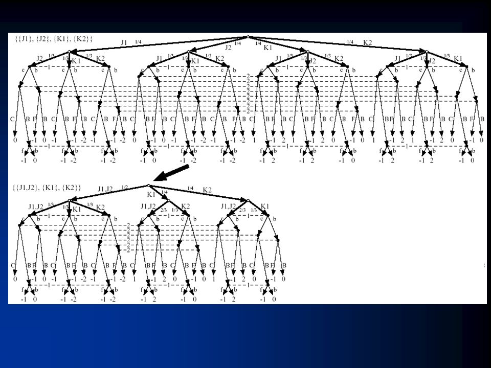
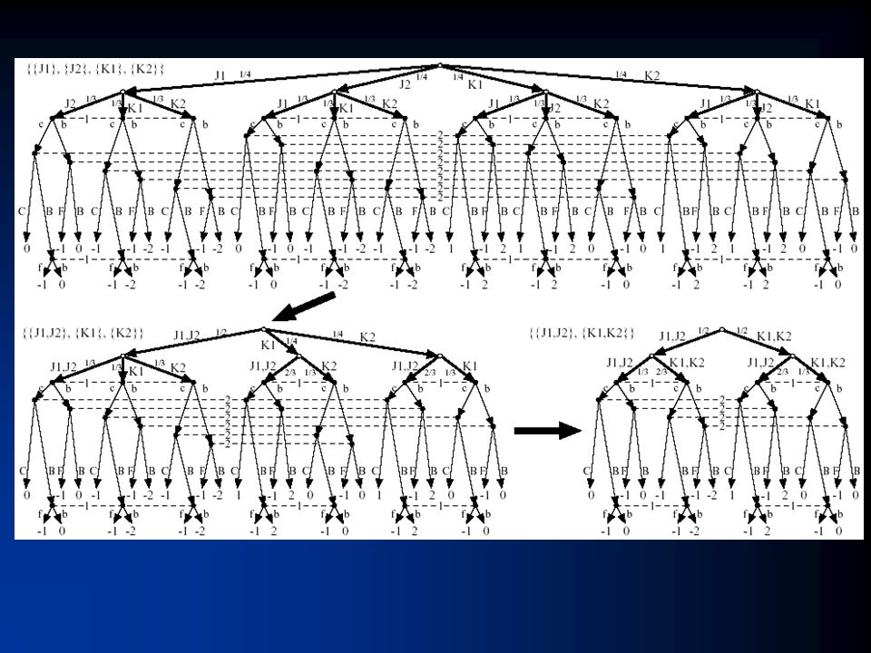
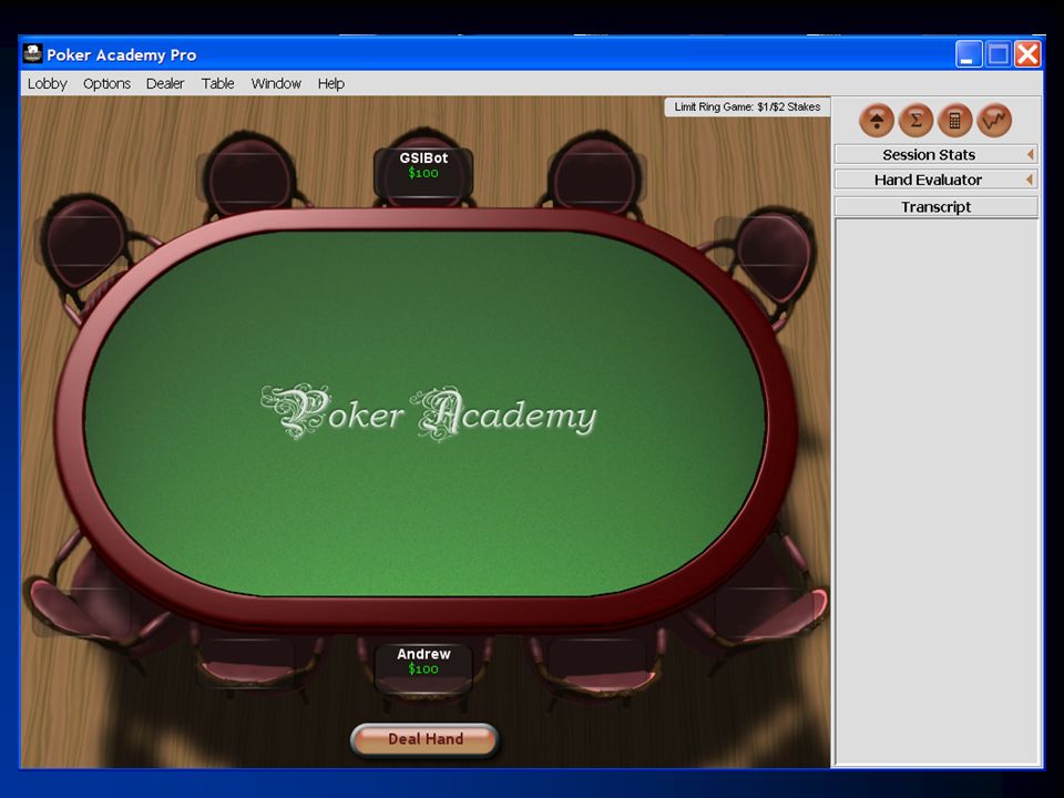
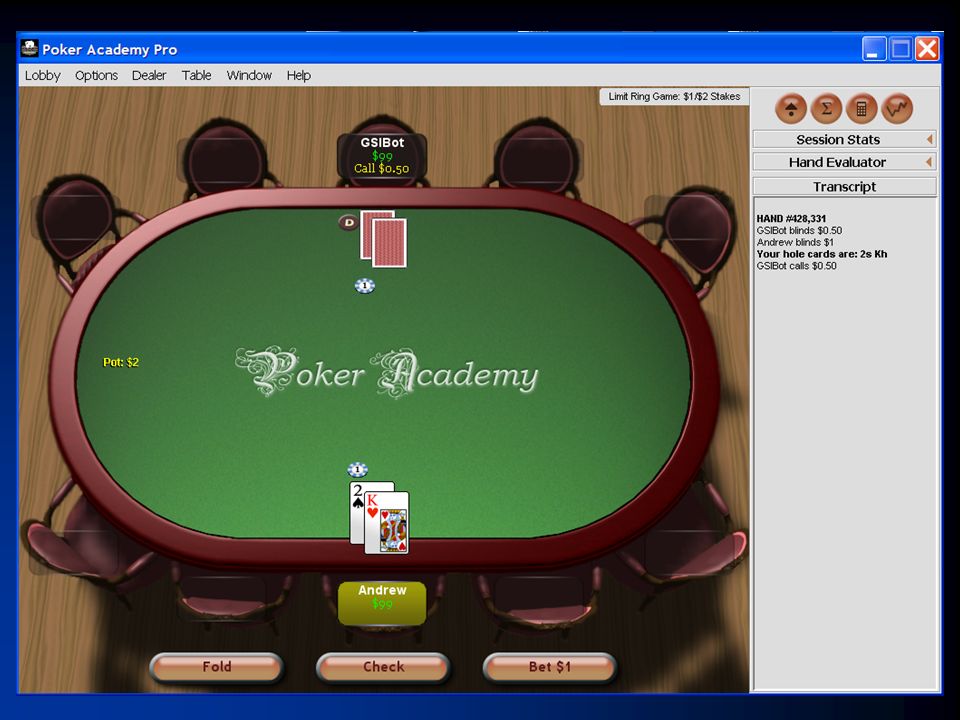

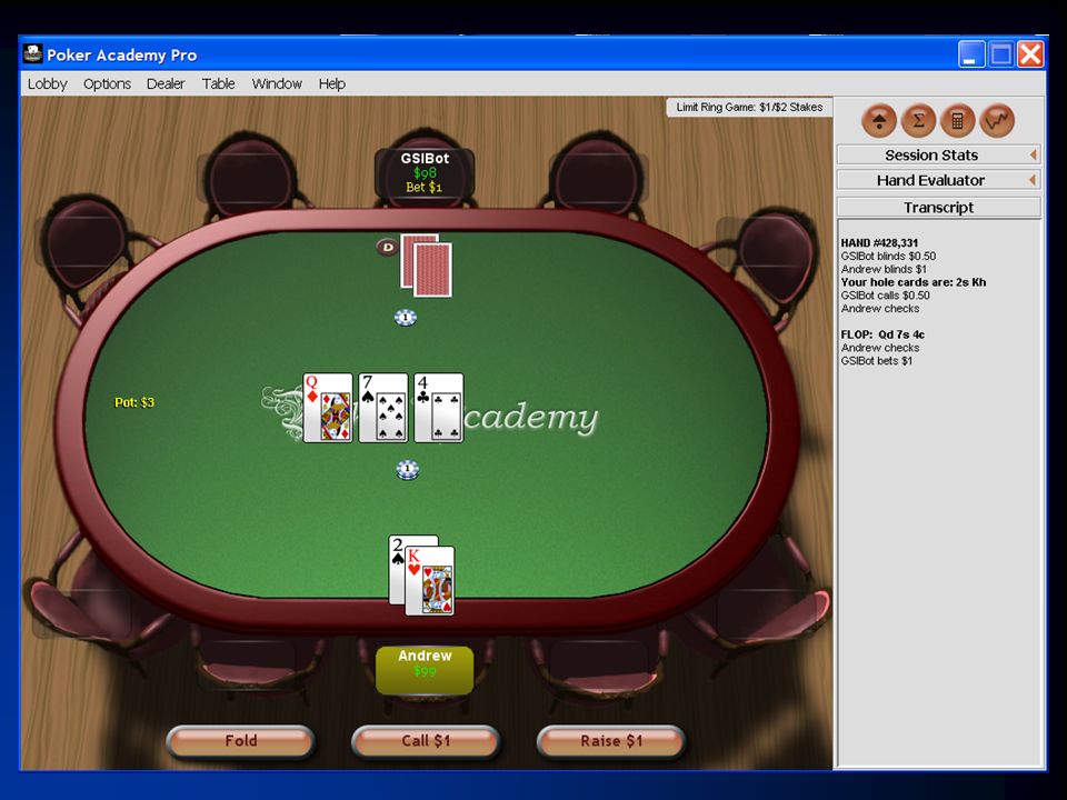

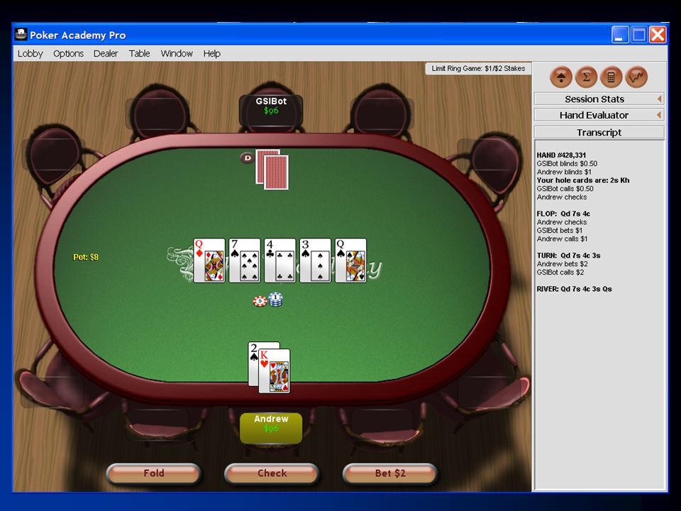

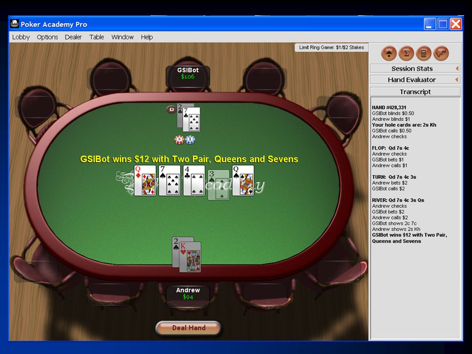

: Every finite game (finite number of players, finite number of pure strategies) has at least one mixed-strategy Nash.>")


>")


 Robert Holte Computing Science Dept. University of Alberta.>")
