Download presentation
Presentation is loading. Please wait.

2
Confounding, Effect Modification, and Stratification

3
Adding a Third Dimension to the RxC picture ExposureDisease ? Mediator Confounder Effect modifier

4
1. Confounding A confounding variable is associated with the exposure and it affects the outcome, but it is not an intermediate link in the chain of causation between exposure and outcome.

5
Confounding: Example

6
Confounding: example Drinker Non-drinker 100200 Lung cancerNo lung cancer 50 150 50% of cases are drinkers, but only 25% of controls are drinkers. Therefore, it appears that drinking is strongly associated with lung cancer.

7
Confounding: example Drinker Non-drinker Lung cancerNo lung cancer 4515 30 10 Drinker Non-drinker Lung cancerNo lung cancer 535 20 140 Smoker Non-smoker Among smokers, 45/75=60% of lung cancer cases drink and 15/25=60% of controls drink. Among non-smokers 5/25=20% of lung cancer cases drink and 35/175=20% of controls drink. 75 25 175

8
Confusion over postmenopausal hormones: Postmenopausal HRT Heart attacks (MI) ? High SES, high education, other confounders?

9
Mixture May Rival Estrogen in Preventing Heart Disease August 15, 1996, Thursday “Widely prescribed hormone pills that combine estrogen and progestin appear to be just as effective as estrogen alone in preventing heart disease in women after menopause, a study has concluded.” “Many women take hormones … to reduce the risk of heart disease and broken bones.” “More than 30 studies have found that estrogen after menopause is good for the heart.”

10
Example: Nurse’s Health Study protective relative risks

11
Nurse’s Health Study

12
No apparent Confounding… e.g., the effect is the same among smokers and non-smokers, so the association couldn’t be due to confounding by smokers (who may take less hormones and certainly get more heart disease).
.")
13
RCT: Women’s Health Initiative (2002) On hormones On placebo
 On hormones On placebo")
14
Controlling for confounders in medical studies 1. Confounders can be controlled for in the design phase of a study (randomization or restriction or matching). 2. Confounders can be controlled for in the analysis phase of a study (stratification or multivariate regression).
. 2. Confounders can be controlled for in the analysis phase of a study (stratification or multivariate regression)..")
15
Analytical identification of confounders through stratification

16
Mantel-Haenszel Procedure: Non-regression technique used to identify confounders and to control for confounding in the statistical analysis phase rather than the design phase of a study.

17
Stratification: “Series of 2x2 tables” Idea: Take a 2x2 table and break it into a series of smaller 2x2 tables (one table at each of J levels of the confounder yields J tables). Example: in testing for an association between lung cancer and alcohol drinking (yes/no), separate smokers and non-smokers.
, separate smokers and non-smokers..")
18
Stratification:“Series of 2xK tables” Idea: Take a 2xK table and break it into a series of smaller 2xK tables (one table at each of J levels of the confounder yields J tables). Example: In evaluating the association between lung cancer and being either a teetotaler, light drinker, moderate drinker, or heavy drinker (2x4 table), separate into smokers and non-smokers (two 2x4 tables).
, separate into smokers and non-smokers (two 2x4 tables)..")
19
Road Map 1.Test for Conditional Independence (Mantel-Haenszel, or “Cochran-Mantel- Haenszel”, Test). Null hypothesis: when conditioned on the confounder, exposure and disease are independent. Mathematically, (for dichotomous confounder): P(E&D/~C) = P(E/~C)*P(D/~C) and P(E&D/C)=P(E/C)*P(D/C) Example: once you condition on smoking, alcohol and lung cancer are independent; M-H test comes out NS. 2. Test for homogeneity. Breslow-Day. Null hypothesis: the relationship (or lack of relationship) between exposure and disease is the same in each stratum (homogeneity). Example: B-D test would come out significant if alcohol aggravated the risk of cigarettes on lung cancer but did not increase lung cancer risk in non-smokers. Homogeneity does NOT require independence!! 3. If homogenous, for series of 2x2 tables, you can take a weighted average of OR’s or RR’s (which should be similar in each stratum !) from the strata to get an overall OR or RR that has been controlled for confounding by C.
: P(E&D/~C) = P(E/~C)*P(D/~C) and P(E&D/C)=P(E/C)*P(D/C) Example: once you condition on smoking, alcohol and lung cancer are independent; M-H test comes out NS. 2. Test for homogeneity. Breslow-Day. Null hypothesis: the relationship (or lack of relationship) between exposure and disease is the same in each stratum (homogeneity). Example: B-D test would come out significant if alcohol aggravated the risk of cigarettes on lung cancer but did not increase lung cancer risk in non-smokers. Homogeneity does NOT require independence!. 3. If homogenous, for series of 2x2 tables, you can take a weighted average of OR’s or RR’s (which should be similar in each stratum !) from the strata to get an overall OR or RR that has been controlled for confounding by C..")
20
Controlling for confounding by stratification Example: Gender Bias at Berkeley? (From: Sex Bias in Graduate Admissions: Data from Berkeley, Science 187: 398-403; 1975.) Crude RR = (1276/1835)/(1486/2681) =1.25 (1.20 – 1.32) Denied Admitted 18352681 FemaleMale 12761486 559 1195
 Crude RR = (1276/1835)/(1486/2681) =1.25 (1.20 – 1.32) Denied Admitted FemaleMale")
21
Program A Stratum 1 = only those who applied to program A Stratum-specific RR =.46 (.30-.70) Denied Admitted 108825 FemaleMale 19314 89 511
 Denied Admitted FemaleMale")
22
Program B Stratum 2 = only those who applied to program B Stratum-specific RR = 0.86 (.48-1.54) Denied Admitted 25560 FemaleMale 8208 17 352
 Denied Admitted FemaleMale")
23
Program C Stratum 3 = only those who applied to program C Stratum-specific RR = 1.05 (.94-1.16) Denied Admitted 593325 FemaleMale 391205 202 120
 Denied Admitted FemaleMale")
24
Program D Stratum 4 = only those who applied to program D Stratum-specific RR = 1.02 (.92-1.12) Denied Admitted 375407 FemaleMale 248265 127 142
 Denied Admitted FemaleMale")
25
Program E Stratum 5 = only those who applied to program E Stratum-specific RR = 0.96 (.87-1.05) Denied Admitted 393191 FemaleMale 289147 104 44
 Denied Admitted FemaleMale")
26
Program F Stratum 6 = only those who applied to program F Stratum-specific RR = 1.01 (.97-1.05) Denied Admitted 341373 FemaleMale 321347 20 26
 Denied Admitted FemaleMale")
27
Summary Crude RR = 1.25 (1.20 – 1.32) Stratum specific RR’s:.46 (.30-.70) 0.86 (.48-1.54) 1.05 (.94-1.16) 1.02 (.92-1.12) 0.96 (.87-1.05) 1.01 (.97-1.05) Maentel-Haenszel Summary RR:.97 Cochran-Mantel-Haenszel Test is NS. Gender and denial of admissions are conditionally independent given program. The apparent association (RR=1.25) was due to confounding.
 was due to confounding..")
28
Cochran-Mantel-Haenszel Test of Conditional Independence The (Cochran)-Mantel-Haenszel statistic tests the null hypothesis that exposure and disease are independent when conditioned on the confounder.
-Mantel-Haenszel statistic tests the null hypothesis that exposure and disease are independent when conditioned on the confounder.")
29
CMH test of conditional independence Exposed Unexposed DiseaseNo Disease ab cd Strata k NkNk

30
CMH test of conditional independence Exposed Unexposed DiseaseNo Disease ab cd Strata k NkNk

31
E.g., for Berkeley… Result is NS

32
Summary Crude RR = 1.25 (1.20 – 1.32) Stratum specific RR’s:.46 (.30-.70) 0.86 (.48-1.54) 1.05 (.94-1.16) 1.02 (.92-1.12) 0.96 (.87-1.05) 1.01 (.97-1.05) Breslow-Day test rejects (p=.0023) because of the protective effect for women in program A. We will still combine them—but that may obscure a potentially interesting pro-female bias in program A!

33
The Mantel-Haenszel Summary Risk Ratio Disease Not Disease ExposureNot Exposed ac b d k strata

34
The Mantel-Haenszel Summary Risk Ratio Disease Not Disease ExposureNot Exposed ac b d total unexposed total exposed Exposed &disease Unexposed&disease

35
The Mantel-Haenszel Summary Risk Ratio Disease Not Disease ExposureNot Exposed ac b d

36
E.g., for Berkeley… Use computer to get confidence limits…

37
The Mantel-Haenszel Summary Odds Ratio Exposed Not Exposed CaseControl ab c d

38
Country OR = 1.32 Spouse smokes Spouse does not smoke 137363 71 249 US Spouse smokes Spouse does not smoke 1938 5 16 Great Britain OR = 1.6 Spouse smokes Spouse does not smoke Lung CancerControl73188 21 82 Japan OR = 1.52 Source: Agresti. Introduction to Categorical Data Analysis. 2007. Chapter 3. Example…

39
In SAS… proc freq data=secondhand; weight number; * specifies the size of each 2x2 cell; tables country*NoSpouse*NotCase/ cmh ; run;

40
CMH test of conditional independence: p=.0196 Summary Statistics for Spouse by Case Controlling for Country Cochran-Mantel-Haenszel Statistics (Based on Table Scores) Statistic Alternative Hypothesis DF Value Prob ƒƒƒƒƒƒƒƒƒƒƒƒƒƒƒƒƒƒƒƒƒƒƒƒƒƒƒƒƒƒƒƒƒƒƒƒƒƒƒƒƒƒƒƒƒƒƒƒƒƒƒƒƒƒƒƒƒƒƒƒƒƒƒ 1 Nonzero Correlation 1 5.4497 0.0196 Significant CMH test means that there does appear to be an association between spousal smoking and cancer, after controlling for country.
 Statistic Alternative Hypothesis DF Value Prob ƒƒƒƒƒƒƒƒƒƒƒƒƒƒƒƒƒƒƒƒƒƒƒƒƒƒƒƒƒƒƒƒƒƒƒƒƒƒƒƒƒƒƒƒƒƒƒƒƒƒƒƒƒƒƒƒƒƒƒƒƒƒƒ 1 Nonzero Correlation Significant CMH test means that there does appear to be an association between spousal smoking and cancer, after controlling for country.")
41
Breslow-Day test of homogeneity: NS Controlling for Country Breslow-Day Test for Homogeneity of the Odds Ratios ƒƒƒƒƒƒƒƒƒƒƒƒƒƒƒƒƒƒƒƒƒƒƒƒƒƒƒƒƒƒ Chi-Square 0.2381 DF Pr > ChiSq 0.8878 Total Sample Size = 1262 NS means there’s no evidence that OR’s differ across strata (OK to combine them into summary OR)
")
42
Summary Statistics for Spouse by Case Controlling for Country Estimates of the Common Relative Risk (Row1/Row2) Type of Study Method Value ƒƒƒƒƒƒƒƒƒƒƒƒƒƒƒƒƒƒƒƒƒƒƒƒƒƒƒƒƒƒƒƒƒƒƒƒƒƒƒƒƒƒƒƒƒƒƒ Case-Control Mantel-Haenszel 1.3854 (Odds Ratio) Logit 1.3839 Cohort Mantel-Haenszel 1.2779 (Col1 Risk) Logit 1.2760 Cohort Mantel-Haenszel 0.9225 (Col2 Risk) Logit 0.9223 Type of Study Method 95% Confidence Limits ƒƒƒƒƒƒƒƒƒƒƒƒƒƒƒƒƒƒƒƒƒƒƒƒƒƒƒƒƒƒƒƒƒƒƒƒƒƒƒƒƒƒƒƒƒƒƒƒƒƒƒƒƒƒƒƒƒƒƒƒƒ Case-Control Mantel-Haenszel 1.0536 1.8217 (Odds Ratio) Logit 1.0521 1.8203 MH OR and confidence limits…
 Type of Study Method Value ƒƒƒƒƒƒƒƒƒƒƒƒƒƒƒƒƒƒƒƒƒƒƒƒƒƒƒƒƒƒƒƒƒƒƒƒƒƒƒƒƒƒƒƒƒƒƒ Case-Control Mantel-Haenszel (Odds Ratio) Logit Cohort Mantel-Haenszel (Col1 Risk) Logit Cohort Mantel-Haenszel (Col2 Risk) Logit Type of Study Method 95% Confidence Limits ƒƒƒƒƒƒƒƒƒƒƒƒƒƒƒƒƒƒƒƒƒƒƒƒƒƒƒƒƒƒƒƒƒƒƒƒƒƒƒƒƒƒƒƒƒƒƒƒƒƒƒƒƒƒƒƒƒƒƒƒƒ Case-Control Mantel-Haenszel (Odds Ratio) Logit MH OR and confidence limits…")
43
Country OR = 1.32 Spouse smokes Spouse does not smoke 137363 71 249 US Spouse smokes Spouse does not smoke 1938 5 16 Great Britain OR = 1.6 Spouse smokes Spouse does not smoke Lung CancerControl73188 21 82 Japan OR = 1.52 Example… Source: Agresti. Introduction to Categorical Data Analysis. 2007. Chapter 3.

44
The Mantel-Haenszel Summary Odds Ratio Exposed Not Exposed CaseControl ab c d

45
Summary OR Not Surprising!

46
MH OR assumptions OR or RR doesn’t vary across strata. (Homogeneity!) If exposure/disease association does vary for different subgroups, then the summary OR or RR is not appropriate…
 If exposure/disease association does vary for different subgroups, then the summary OR or RR is not appropriate….")
47
advantages and limitations advantages… Mantel-Haenszel summary statistic is easy to interpret and calculate Gives you a hands-on feel for the data disadvantages… Requires categorical confounders or continuous confounders that have been divided into intervals Cumbersome if more than a single confounder To control for 1 and/or continuous confounders, a multivariate technique (such as logistic regression) is preferable.
 is preferable.")
48
2. Effect Modification Effect modification occurs when the effect of an exposure is different among different subgroups.

49
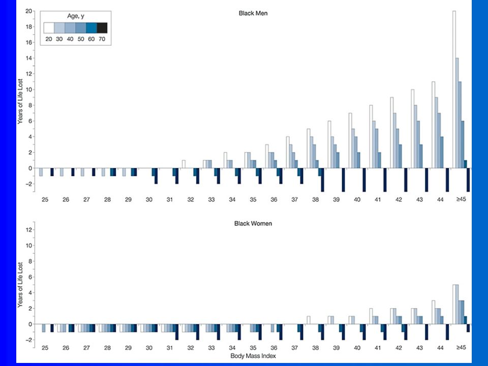
Years of Life Lost Due to Obesity (JAMA. Jan 8 2003;289:187-193) Data from US Life Tables and the National Health and Nutrition Examination Surveys (I, II, III).
 Data from US Life Tables and the National Health and Nutrition Examination Surveys (I, II, III)..")
52
Conclusion Race and gender modify the effect of obesity on years-of-life-lost.

53
Among white women, stage of breast cancer at detection is associated with education. However, no clear pattern among black women.

54
Colon cancer and obesity in pre- and post-menopausal women Obesity appears to be a risk factor in pre- menopausal women But appears to be protective or unrelated in post-menopausal women

Similar presentations

>")


 19.3 Mantel-Haenszel Methods 19.4 Interaction.>")


