2. Econ 482 Lecture 1 I. Administration: Introduction Syllabus Thursday, Jan 16 th, “Lab” class is from 5-6pm in Savery 117 II. Material: Start of Statistical Review: Discrete and continuous random variables Expected value, variance

3. Random variables: A random variable is any variable whose value cannot be predicted exactly 1.Discrete random variables: Random variable which has a specific (countable set) of possible values Examples? 2. Continuous random variables: Random variable which can take any value of a continuous range of values

4. Properties of discrete random variables

5. © Christopher Dougherty 1999–2006 PROBABILITY DISTRIBUTION EXAMPLE: X IS THE SUM OF TWO DICE red123456 This sequence provides an example of a discrete random variable. Suppose that you have a red die which, when thrown, takes the numbers from 1 to 6 with equal probability.

6. © Christopher Dougherty 1999–2006 red123456 green 1 2 3 4 5 6 Suppose that you also have a green die that can take the numbers from 1 to 6 with equal probability. PROBABILITY DISTRIBUTION EXAMPLE: X IS THE SUM OF TWO DICE

7. © Christopher Dougherty 1999–2006 red123456 green 1 2 3 4 5 6 We will define a random variable X as the sum of the numbers when the dice are thrown. PROBABILITY DISTRIBUTION EXAMPLE: X IS THE SUM OF TWO DICE

8. © Christopher Dougherty 1999–2006 For example, if the red die is 4 and the green one is 6, X is equal to 10. red123456 green 1 2 3 4 5 6 10 PROBABILITY DISTRIBUTION EXAMPLE: X IS THE SUM OF TWO DICE

9. © Christopher Dougherty 1999–2006 red123456 green 1 2 3 4 57 6 Similarly, if the red die is 2 and the green one is 5, X is equal to 7. PROBABILITY DISTRIBUTION EXAMPLE: X IS THE SUM OF TWO DICE

10. © Christopher Dougherty 1999–2006 red123456 green 1234567 2345678 3456789 45678910 567891011 6789101112 The table shows all the possible outcomes. PROBABILITY DISTRIBUTION EXAMPLE: X IS THE SUM OF TWO DICE

11. © Christopher Dougherty 1999–2006 red123456 green 1234567 2345678 3456789 45678910 567891011 6789101112 X 2 3 4 5 6 7 8 9 10 11 12 If you look at the table, you can see that X can be any of the numbers from 2 to 12. PROBABILITY DISTRIBUTION EXAMPLE: X IS THE SUM OF TWO DICE

12. © Christopher Dougherty 1999–2006 red123456 green 1234567 2345678 3456789 45678910 567891011 6789101112 Xf 2 3 4 5 6 7 8 9 10 11 12 We will now define f, the frequencies associated with the possible values of X. PROBABILITY DISTRIBUTION EXAMPLE: X IS THE SUM OF TWO DICE

13. © Christopher Dougherty 1999–2006 red123456 green 1234567 2345678 3456789 45678910 567891011 6789101112 Xf 2 3 4 54 6 7 8 9 10 11 12 For example, there are four outcomes which make X equal to 5. PROBABILITY DISTRIBUTION EXAMPLE: X IS THE SUM OF TWO DICE

14. © Christopher Dougherty 1999–2006 red123456 green 1234567 2345678 3456789 45678910 567891011 6789101112 Xf 21 32 43 54 65 76 85 94 103 112 121 Similarly you can work out the frequencies for all the other values of X. PROBABILITY DISTRIBUTION EXAMPLE: X IS THE SUM OF TWO DICE

15. © Christopher Dougherty 1999–2006 red123456 green 1234567 2345678 3456789 45678910 567891011 6789101112 Xfp 21 32 43 54 65 76 85 94 103 112 121 Finally we will derive the probability of obtaining each value of X. PROBABILITY DISTRIBUTION EXAMPLE: X IS THE SUM OF TWO DICE

16. © Christopher Dougherty 1999–2006 red123456 green 1234567 2345678 3456789 45678910 567891011 6789101112 Xfp 21 32 43 54 65 76 85 94 103 112 121 If there is 1/6 probability of obtaining each number on the red die, and the same on the green die, each outcome in the table will occur with 1/36 probability. PROBABILITY DISTRIBUTION EXAMPLE: X IS THE SUM OF TWO DICE

17. © Christopher Dougherty 1999–2006 red123456 green 1234567 2345678 3456789 45678910 567891011 6789101112 Xfp 211/36 322/36 433/36 544/36 655/36 766/36 855/36 944/36 1033/36 1122/36 1211/36 Hence to obtain the probabilities associated with the different values of X, we divide the frequencies by 36. PROBABILITY DISTRIBUTION EXAMPLE: X IS THE SUM OF TWO DICE

18. © Christopher Dougherty 1999–2006 The distribution is shown graphically. in this example it is symmetrical, highest for X equal to 7 and declining on either side. 6 __ 36 5 __ 36 4 __ 36 3 __ 36 2 __ 36 2 __ 36 3 __ 36 5 __ 36 4 __ 36 probability 23 456789101112 X PROBABILITY DISTRIBUTION EXAMPLE: X IS THE SUM OF TWO DICE 1 36 1 36

19. © Christopher Dougherty 1999–2006 Definition of E(X), the expected value of X: EXPECTED VALUE OF A RANDOM VARIABLE The expected value of a random variable, also known as its population mean, is the weighted average of its possible values, the weights being the probabilities attached to the values.

20. © Christopher Dougherty 1999–2006 Definition of E(X), the expected value of X: EXPECTED VALUE OF A RANDOM VARIABLE Note that the sum of the probabilities must be unity, so there is no need to divide by the sum of the weights.

21. © Christopher Dougherty 1999–2006 x i x 1 x 2 x 3 x 4 x 5 x 6 x 7 x 8 x 9 x 10 x 11 EXPECTED VALUE OF A RANDOM VARIABLE This sequence shows how the expected value is calculated, first in abstract and then with the random variable defined in the first sequence. We begin by listing the possible values of X.

22. © Christopher Dougherty 1999–2006 x i p i x 1 p 1 x 2 p 2 x 3 p 3 x 4 p 4 x 5 p 5 x 6 p 6 x 7 p 7 x 8 p 8 x 9 p 9 x 10 p 10 x 11 p 11 EXPECTED VALUE OF A RANDOM VARIABLE Next we list the probabilities attached to the different possible values of X.

23. © Christopher Dougherty 1999–2006 x i p i x 1 p 1 x 2 p 2 x 3 p 3 x 4 p 4 x 5 p 5 x 6 p 6 x 7 p 7 x 8 p 8 x 9 p 9 x 10 p 10 x 11 p 11 EXPECTED VALUE OF A RANDOM VARIABLE Then we define a column in which the values are weighted by the corresponding probabilities.

24. © Christopher Dougherty 1999–2006 x i p i x 1 p 1 x 2 p 2 x 3 p 3 x 4 p 4 x 5 p 5 x 6 p 6 x 7 p 7 x 8 p 8 x 9 p 9 x 10 p 10 x 11 p 11 EXPECTED VALUE OF A RANDOM VARIABLE We do this for each value separately.

25. © Christopher Dougherty 1999–2006 x i p i x 1 p 1 x 2 p 2 x 3 p 3 x 4 p 4 x 5 p 5 x 6 p 6 x 7 p 7 x 8 p 8 x 9 p 9 x 10 p 10 x 11 p 11 EXPECTED VALUE OF A RANDOM VARIABLE Here we are assuming that n, the number of possible values, is equal to 11, but it could be any number.

26. © Christopher Dougherty 1999–2006 x i p i x 1 p 1 x 2 p 2 x 3 p 3 x 4 p 4 x 5 p 5 x 6 p 6 x 7 p 7 x 8 p 8 x 9 p 9 x 10 p 10 x 11 p 11  x i p i = E(X) EXPECTED VALUE OF A RANDOM VARIABLE The expected value is the sum of the entries in the third column.

27. © Christopher Dougherty 1999–2006 x i p i x i p i x i p i x 1 p 1 x 1 p 1 21/36 x 2 p 2 x 2 p 2 32/36 x 3 p 3 x 3 p 3 43/36 x 4 p 4 x 4 p 4 54/36 x 5 p 5 x 5 p 5 65/36 x 6 p 6 x 6 p 6 76/36 x 7 p 7 x 7 p 7 85/36 x 8 p 8 x 8 p 8 94/36 x 9 p 9 x 9 p 9 103/36 x 10 p 10 x 10 p 10 112/36 x 11 p 11 x 11 p 11 121/36  x i p i = E(X) EXPECTED VALUE OF A RANDOM VARIABLE The random variable X defined in the previous sequence could be any of the integers from 2 to 12 with probabilities as shown.

28. © Christopher Dougherty 1999–2006 x i p i x i p i x 1 p 1 x 1 p 1 21/362/36 x 2 p 2 x 2 p 2 32/36 x 3 p 3 x 3 p 3 43/36 x 4 p 4 x 4 p 4 54/36 x 5 p 5 x 5 p 5 65/36 x 6 p 6 x 6 p 6 76/36 x 7 p 7 x 7 p 7 85/36 x 8 p 8 x 8 p 8 94/36 x 9 p 9 x 9 p 9 103/36 x 10 p 10 x 10 p 10 112/36 x 11 p 11 x 11 p 11 121/36  x i p i = E(X) EXPECTED VALUE OF A RANDOM VARIABLE X could be equal to 2 with probability 1/36, so the first entry in the calculation of the expected value is 2/36.

29. © Christopher Dougherty 1999–2006 x i p i x i p i x 1 p 1 x 1 p 1 21/362/36 x 2 p 2 x 2 p 2 32/366/36 x 3 p 3 x 3 p 3 43/36 x 4 p 4 x 4 p 4 54/36 x 5 p 5 x 5 p 5 65/36 x 6 p 6 x 6 p 6 76/36 x 7 p 7 x 7 p 7 85/36 x 8 p 8 x 8 p 8 94/36 x 9 p 9 x 9 p 9 103/36 x 10 p 10 x 10 p 10 112/36 x 11 p 11 x 11 p 11 121/36  x i p i = E(X) EXPECTED VALUE OF A RANDOM VARIABLE The probability of x being equal to 3 was 2/36, so the second entry is 6/36.

30. © Christopher Dougherty 1999–2006 x i p i x i p i x 1 p 1 x 1 p 1 21/362/36 x 2 p 2 x 2 p 2 32/366/36 x 3 p 3 x 3 p 3 43/3612/36 x 4 p 4 x 4 p 4 54/3620/36 x 5 p 5 x 5 p 5 65/3630/36 x 6 p 6 x 6 p 6 76/3642/36 x 7 p 7 x 7 p 7 85/3640/36 x 8 p 8 x 8 p 8 94/3636/36 x 9 p 9 x 9 p 9 103/3630/36 x 10 p 10 x 10 p 10 112/3622/36 x 11 p 11 x 11 p 11 121/3612/36  x i p i = E(X) EXPECTED VALUE OF A RANDOM VARIABLE Similarly for the other 9 possible values.

31. © Christopher Dougherty 1999–2006 x i p i x i p i x 1 p 1 x 1 p 1 21/362/36 x 2 p 2 x 2 p 2 32/366/36 x 3 p 3 x 3 p 3 43/3612/36 x 4 p 4 x 4 p 4 54/3620/36 x 5 p 5 x 5 p 5 65/3630/36 x 6 p 6 x 6 p 6 76/3642/36 x 7 p 7 x 7 p 7 85/3640/36 x 8 p 8 x 8 p 8 94/3636/36 x 9 p 9 x 9 p 9 103/3630/36 x 10 p 10 x 10 p 10 112/3622/36 x 11 p 11 x 11 p 11 121/3612/36  x i p i = E(X) 252/36 To obtain the expected value, we sum the entries in this column. EXPECTED VALUE OF A RANDOM VARIABLE

32. © Christopher Dougherty 1999–2006 The expected value turns out to be 7. Actually, this was obvious anyway. We saw in the previous sequence that the distribution is symmetrical about 7. EXPECTED VALUE OF A RANDOM VARIABLE x i p i x i p i x 1 p 1 x 1 p 1 21/362/36 x 2 p 2 x 2 p 2 32/366/36 x 3 p 3 x 3 p 3 43/3612/36 x 4 p 4 x 4 p 4 54/3620/36 x 5 p 5 x 5 p 5 65/3630/36 x 6 p 6 x 6 p 6 76/3642/36 x 7 p 7 x 7 p 7 85/3640/36 x 8 p 8 x 8 p 8 94/3636/36 x 9 p 9 x 9 p 9 103/3630/36 x 10 p 10 x 10 p 10 112/3622/36 x 11 p 11 x 11 p 11 121/3612/36  x i p i = E(X) 252/36 = 7

33. © Christopher Dougherty 1999–2006 Alternative notation for E(X): E(X) =  X Very often the expected value of a random variable is represented by , the Greek m. If there is more than one random variable, their expected values are differentiated by adding subscripts to . EXPECTED VALUE OF A RANDOM VARIABLE

34. © Christopher Dougherty 1999–2006 Definition of E[g(X)], the expected value of a function of X: To find the expected value of a function of a random variable, you calculate all the possible values of the function, weight them by the corresponding probabilities, and sum the results. EXPECTED VALUE OF A FUNCTION OF A RANDOM VARIABLE

35. © Christopher Dougherty 1999–2006 Definition of E[g(X)], the expected value of a function of X: Example: For example, the expected value of X 2 is found by calculating all its possible values, multiplying them by the corresponding probabilities, and summing. EXPECTED VALUE OF A FUNCTION OF A RANDOM VARIABLE

36. © Christopher Dougherty 1999–2006 xipix1p1x2p2x3p3……………………………………xnpn xipix1p1x2p2x3p3……………………………………xnpn ………………… First you list the possible values of X and the corresponding probabilities. EXPECTED VALUE OF A FUNCTION OF A RANDOM VARIABLE

37. © Christopher Dougherty 1999–2006 x i p i g(x i ) x 1 p 1 g(x 1 ) x 2 p 2 g(x 2 ) x 3 p 3 g(x 3 ) ………... x n p n g(x n ) Next you calculate the function of X for each possible value of X. EXPECTED VALUE OF A FUNCTION OF A RANDOM VARIABLE

38. © Christopher Dougherty 1999–2006 x i p i g(x i ) g(x i ) p i x 1 p 1 g(x 1 )g(x 1 ) p 1 x 2 p 2 g(x 2 ) x 3 p 3 g(x 3 ) ………... x n p n g(x n ) Then, one at a time, you weight the value of the function by its corresponding probability. EXPECTED VALUE OF A FUNCTION OF A RANDOM VARIABLE

39. © Christopher Dougherty 1999–2006 x i p i g(x i ) g(x i ) p i x 1 p 1 g(x 1 )g(x 1 ) p 1 x 2 p 2 g(x 2 ) g(x 2 ) p 2 x 3 p 3 g(x 3 ) g(x 3 ) p 3 ………...……... x n p n g(x n ) g(x n ) p n You do this individually for each possible value of X. EXPECTED VALUE OF A FUNCTION OF A RANDOM VARIABLE

40. © Christopher Dougherty 1999–2006 x i p i g(x i ) g(x i ) p i x 1 p 1 g(x 1 )g(x 1 ) p 1 x 2 p 2 g(x 2 ) g(x 2 ) p 2 x 3 p 3 g(x 3 ) g(x 3 ) p 3 ………...……... x n p n g(x n ) g(x n ) p n   g(x i ) p i The sum of the weighted values is the expected value of the function of X. EXPECTED VALUE OF A FUNCTION OF A RANDOM VARIABLE

41. © Christopher Dougherty 1999–2006 x i p i g(x i ) g(x i ) p i x i p i x 1 p 1 g(x 1 )g(x 1 ) p 1 21/36 x 2 p 2 g(x 2 ) g(x 2 ) p 2 32/36 x 3 p 3 g(x 3 ) g(x 3 ) p 3 43/36 ………...……... 54/36 ………...……... 65/36 ………...……... 76/36 ………...……... 85/36 ………...……... 94/36 ………...……... 103/36 ………...……... 112/36 x n p n g(x n ) g(x n ) p n 121/36   g(x i ) p i The process will be illustrated for X 2, where X is the random variable defined in the first sequence. The 11 possible values of X and the corresponding probabilities are listed. EXPECTED VALUE OF A FUNCTION OF A RANDOM VARIABLE

42. © Christopher Dougherty 1999–2006 x i p i g(x i ) g(x i ) p i x i p i x i 2 x 1 p 1 g(x 1 )g(x 1 ) p 1 21/364 x 2 p 2 g(x 2 ) g(x 2 ) p 2 32/369 x 3 p 3 g(x 3 ) g(x 3 ) p 3 43/3616 ………...……... 54/3625 ………...……... 65/3636 ………...……... 76/3649 ………...……... 85/3664 ………...……... 94/3681 ………...……... 103/36100 ………...……... 112/36121 x n p n g(x n ) g(x n ) p n 121/36144   g(x i ) p i First you calculate the possible values of X 2. EXPECTED VALUE OF A FUNCTION OF A RANDOM VARIABLE

43. © Christopher Dougherty 1999–2006 x i p i g(x i ) g(x i ) p i x i p i x i 2 x i 2 p i x 1 p 1 g(x 1 )g(x 1 ) p 1 21/3640.11 x 2 p 2 g(x 2 ) g(x 2 ) p 2 32/369 x 3 p 3 g(x 3 ) g(x 3 ) p 3 43/3616 ………...……... 54/3625 ………...……... 65/3636 ………...……... 76/3649 ………...……... 85/3664 ………...……... 94/3681 ………...……... 103/36100 ………...……... 112/36121 x n p n g(x n ) g(x n ) p n 121/36144   g(x i ) p i The first value is 4, which arises when X is equal to 2. The probability of X being equal to 2 is 1/36, so the weighted function is 4/36, which we shall write in decimal form as 0.11. EXPECTED VALUE OF A FUNCTION OF A RANDOM VARIABLE

44. © Christopher Dougherty 1999–2006 x i p i g(x i ) g(x i ) p i x i p i x i 2 x i 2 p i x 1 p 1 g(x 1 )g(x 1 ) p 1 21/3640.11 x 2 p 2 g(x 2 ) g(x 2 ) p 2 32/3690.50 x 3 p 3 g(x 3 ) g(x 3 ) p 3 43/36161.33 ………...……... 54/36252.78 ………...……... 65/36365.00 ………...……... 76/36498.17 ………...……... 85/36648.89 ………...……... 94/36819.00 ………...……... 103/361008.83 ………...……... 112/361216.72 x n p n g(x n ) g(x n ) p n 121/361444.00   g(x i ) p i Similarly for all the other possible values of X. EXPECTED VALUE OF A FUNCTION OF A RANDOM VARIABLE

45. © Christopher Dougherty 1999–2006 x i p i g(x i ) g(x i ) p i x i p i x i 2 x i 2 p i x 1 p 1 g(x 1 )g(x 1 ) p 1 21/3640.11 x 2 p 2 g(x 2 ) g(x 2 ) p 2 32/3690.50 x 3 p 3 g(x 3 ) g(x 3 ) p 3 43/36161.33 ………...……... 54/36252.78 ………...……... 65/36365.00 ………...……... 76/36498.17 ………...……... 85/36648.89 ………...……... 94/36819.00 ………...……... 103/361008.83 ………...……... 112/361216.72 x n p n g(x n ) g(x n ) p n 121/361444.00   g(x i ) p i 54.83 The expected value of X 2 is the sum of its weighted values in the final column. It is equal to 54.83. It is the average value of the figures in the previous column, taking the differing probabilities into account. EXPECTED VALUE OF A FUNCTION OF A RANDOM VARIABLE

46. © Christopher Dougherty 1999–2006 x i p i g(x i ) g(x i ) p i x i p i x i 2 x i 2 p i x 1 p 1 g(x 1 )g(x 1 ) p 1 21/3640.11 x 2 p 2 g(x 2 ) g(x 2 ) p 2 32/3690.50 x 3 p 3 g(x 3 ) g(x 3 ) p 3 43/36161.33 ………...……... 54/36252.78 ………...……... 65/36365.00 ………...……... 76/36498.17 ………...……... 85/36648.89 ………...……... 94/36819.00 ………...……... 103/361008.83 ………...……... 112/361216.72 x n p n g(x n ) g(x n ) p n 121/361444.00   g(x i ) p i 54.83 Note that E(X 2 ) is not the same thing as E(X), squared. In the previous sequence we saw that E(X) for this example was 7. Its square is 49.

47. © Christopher Dougherty 1999–2006 Population variance of X: The previous sequence defined the expected value of a function of a random variable X. There is only one function that is of much interest to us, at least initially: the squared deviation from the population mean. The expected value of the squared deviation is known as the population variance of X. It is a measure of the dispersion of the distribution of X about its population mean. POPULATION VARIANCE OF A DISCRETE RANDOM VARIABLE

48. © Christopher Dougherty 1999–2006 We will calculate the population variance of the random variable X defined in the first sequence. We start as usual by listing the possible values of X and the corresponding probabilities. POPULATION VARIANCE OF A DISCRETE RANDOM VARIABLE x i p i x i –  (x i –  ) 2 (x i –  ) 2 p i 21/36–5250.69 32/36–4160.89 43/36–390.75 54/36–240.44 65/36–110.14 76/36000.00 85/36110.14 94/36240.44 103/36390.75 112/364160.89 121/365250.69 5.83

49. © Christopher Dougherty 1999–2006 Next we need a column giving the deviations of the possible values of X about its population mean. In the second sequence we saw that the population mean of X was 7. POPULATION VARIANCE OF A DISCRETE RANDOM VARIABLE x i p i x i –  (x i –  ) 2 (x i –  ) 2 p i 21/36–5250.69 32/36–4160.89 43/36–390.75 54/36–240.44 65/36–110.14 76/36000.00 85/36110.14 94/36240.44 103/36390.75 112/364160.89 121/365250.69 5.83

50. © Christopher Dougherty 1999–2006 When X is equal to 2, the deviation is –5. POPULATION VARIANCE OF A DISCRETE RANDOM VARIABLE x i p i x i –  (x i –  ) 2 (x i –  ) 2 p i 21/36–5250.69 32/36–4160.89 43/36–390.75 54/36–240.44 65/36–110.14 76/36000.00 85/36110.14 94/36240.44 103/36390.75 112/364160.89 121/365250.69 5.83

51. © Christopher Dougherty 1999–2006 POPULATION VARIANCE OF A DISCRETE RANDOM VARIABLE x i p i x i –  (x i –  ) 2 (x i –  ) 2 p i 21/36–5250.69 32/36–4160.89 43/36–390.75 54/36–240.44 65/36–110.14 76/36000.00 85/36110.14 94/36240.44 103/36390.75 112/364160.89 121/365250.69 5.83

52. © Christopher Dougherty 1999–2006 Next we need a column giving the squared deviations. When X is equal to 2, the squared deviation is 25. POPULATION VARIANCE OF A DISCRETE RANDOM VARIABLE x i p i x i –  (x i –  ) 2 (x i –  ) 2 p i 21/36–5250.69 32/36–4160.89 43/36–390.75 54/36–240.44 65/36–110.14 76/36000.00 85/36110.14 94/36240.44 103/36390.75 112/364160.89 121/365250.69 5.83

53. © Christopher Dougherty 1999–2006 Similarly for the other values of X. POPULATION VARIANCE OF A DISCRETE RANDOM VARIABLE x i p i x i –  (x i –  ) 2 (x i –  ) 2 p i 21/36–5250.69 32/36–4160.89 43/36–390.75 54/36–240.44 65/36–110.14 76/36000.00 85/36110.14 94/36240.44 103/36390.75 112/364160.89 121/365250.69 5.83

54. © Christopher Dougherty 1999–2006 POPULATION VARIANCE OF A DISCRETE RANDOM VARIABLE x i p i x i –  (x i –  ) 2 (x i –  ) 2 p i 21/36–5250.69 32/36–4160.89 43/36–390.75 54/36–240.44 65/36–110.14 76/36000.00 85/36110.14 94/36240.44 103/36390.75 112/364160.89 121/365250.69 5.83 Now we start weighting the squared deviations by the corresponding probabilities. What do you think the weighted average will be? Have a guess.

55. © Christopher Dougherty 1999–2006 A reason for making an initial guess is that it may help you to identify an arithmetical error, if you make one. If the initial guess and the outcome are very different, that is a warning. POPULATION VARIANCE OF A DISCRETE RANDOM VARIABLE x i p i x i –  (x i –  ) 2 (x i –  ) 2 p i 21/36–5250.69 32/36–4160.89 43/36–390.75 54/36–240.44 65/36–110.14 76/36000.00 85/36110.14 94/36240.44 103/36390.75 112/364160.89 121/365250.69 5.83

56. © Christopher Dougherty 1999–2006 We calculate all the weighted squared deviations. POPULATION VARIANCE OF A DISCRETE RANDOM VARIABLE x i p i x i –  (x i –  ) 2 (x i –  ) 2 p i 21/36–5250.69 32/36–4160.89 43/36–390.75 54/36–240.44 65/36–110.14 76/36000.00 85/36110.14 94/36240.44 103/36390.75 112/364160.89 121/365250.69 5.83

57. © Christopher Dougherty 1999–2006 x i p i x i –  (x i –  ) 2 (x i –  ) 2 p i 21/36–5250.69 32/36–4160.89 43/36–390.75 54/36–240.44 65/36–110.14 76/36000.00 85/36110.14 94/36240.44 103/36390.75 112/364160.89 121/365250.69 5.83 The sum is the population variance of X. POPULATION VARIANCE OF A DISCRETE RANDOM VARIABLE

58. © Christopher Dougherty 1999–2006 Population variance of X In equations, the population variance of X is usually written  X 2,  being the Greek s. POPULATION VARIANCE OF A DISCRETE RANDOM VARIABLE

59. © Christopher Dougherty 1999–2006 Standard deviation of X The standard deviation of X is the square root of its population variance. Usually written  x, it is an alternative measure of dispersion. It has the same units as X. POPULATION VARIANCE OF A DISCRETE RANDOM VARIABLE

60. Properties of continuous random variables

61. © Christopher Dougherty 1999–2006 CONTINUOUS RANDOM VARIABLES A discrete random variable is one that can take only a finite set of values. The sum of the numbers when two dice are thrown is an example. Each value has associated with it a finite probability, which you can think of as a ‘packet’ of probability. The packets sum to unity because the variable must take one of the values. 6 __ 36 5 __ 36 4 __ 36 3 __ 36 2 __ 36 2 __ 36 3 __ 36 5 __ 36 4 __ 36 probability 23 456789101112X 1 36 1 36

62. © Christopher Dougherty 1999–2006 55 607075 X 65 CONTINUOUS RANDOM VARIABLES height However, most random variables encountered in econometrics are continuous. They can take any one of an infinite set of values defined over a range (or possibly, ranges). As a simple example, take the temperature in a room. We will assume that it can be anywhere from 55 to 75 degrees Fahrenheit with equal probability within the range.

63. © Christopher Dougherty 1999–2006 55 607075 X 65 CONTINUOUS RANDOM VARIABLES height In the case of a continuous random variable, the probability of it being equal to a given finite value (for example, temperature equal to 55.473927) is always infinitesimal. For this reason, you can only talk about the probability of a continuous random variable lying between two given values. The probability is represented graphically as an area.

64. © Christopher Dougherty 1999–2006 55 607075 X 65 CONTINUOUS RANDOM VARIABLES 7 height 56 For example, you could measure the probability of the temperature being between 55 and 56, both measured exactly. Given that the temperature lies anywhere between 55 and 75 with equal probability, the probability of it lying between 55 and 56 must be 0.05.

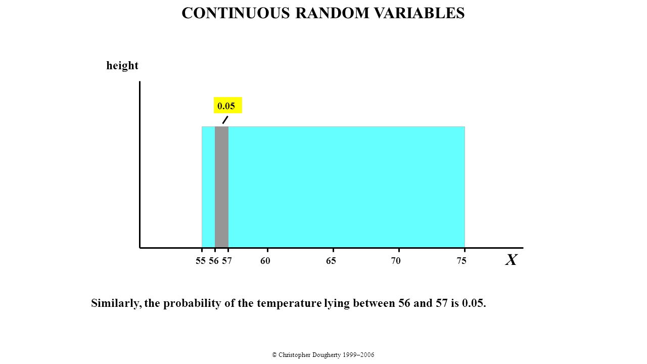
65. © Christopher Dougherty 1999–2006 55 607075 X 65 CONTINUOUS RANDOM VARIABLES 57 height Similarly, the probability of the temperature lying between 56 and 57 is 0.05. 56 0.05

66. © Christopher Dougherty 1999–2006 55 607075 X 65 CONTINUOUS RANDOM VARIABLES 57 58 height And similarly for all the other one-degree intervals within the range. 0.05

67. © Christopher Dougherty 1999–2006 55 607075 X 65 0.05 CONTINUOUS RANDOM VARIABLES 57 58 height The probability per unit interval is 0.05 and accordingly the area of the rectangle representing the probability of the temperature lying in any given unit interval is 0.05. The probability per unit interval is called the probability density and it is equal to the height of the unit-interval rectangle.

68. © Christopher Dougherty 1999–2006 55 607075 X 65 0.05 CONTINUOUS RANDOM VARIABLES f(X) = 0.05 for 55 X 75 f(X) = 0 for X 75 57 58 Mathematically, the probability density is written as a function of the variable, for example f(X). In this example, f(X) is 0.05 for 55 < X < 75 and it is zero elsewhere. height

69. © Christopher Dougherty 1999–2006 55 607075 X 65 0.05 CONTINUOUS RANDOM VARIABLES probability density f(X)f(X) f(X) = 0.05 for 55 X 75 f(X) = 0 for X 75 57 58 The vertical axis is given the label probability density, rather than height. f(X) is known as the probability density function and is shown graphically in the diagram as the thick black line.

70. © Christopher Dougherty 1999–2006 55 607075 X 65 0.05 CONTINUOUS RANDOM VARIABLES probability density f(X)f(X) f(X) = 0.05 for 55 X 75 f(X) = 0 for X 75 Suppose that you wish to calculate the probability of the temperature lying between 65 and 70 degrees. To do this, you should calculate the area under the probability density function between 65 and 70. Typically you have to use the integral calculus to work out the area under a curve, but in this very simple example all you have to do is calculate the area of a rectangle.

71. © Christopher Dougherty 1999–2006 55 607075 X 65 0.05 CONTINUOUS RANDOM VARIABLES The height of the rectangle is 0.05 and its width is 5, so its area is 0.25. probability density f(X)f(X) 0.05 5 0.25 f(X) = 0.05 for 55 X 75 f(X) = 0 for X 75