1. Lecture series: Data analysis Lectures: Each Tuesday at 16:00 (First lecture: May 21, last lecture: June 25) Thomas Kreuz, ISC, CNR thomas.kreuz@cnr.it http://www.fi.isc.cnr.it/users/thomas.kreuz/

2. Lecture 1: Example (Epilepsy & spike train synchrony), Data acquisition, Dynamical systems Lecture 2: Linear measures, Introduction to non-linear dynamics Lecture 3: Non-linear measures Lecture 4: Measures of continuous synchronization (EEG) Lecture 5: Application to non-linear model systems and to epileptic seizure prediction, Surrogates Lecture 6: Measures of (multi-neuron) spike train synchrony (Very preliminary) Schedule

3. Example: Epileptic seizure prediction Data acquisition Introduction to dynamical systems Last lecture

4. Epileptic seizure prediction Epilepsy results from abnormal, hypersynchronous neuronal activity in the brain Accessible brain time series: EEG (standard) and neuronal spike trains (recent) Does a pre-ictal state exist (ictus = seizure)? Do characterizing measures allow a reliable detection of this state? Specific example for prediction of extreme events

5. Data acquisition Sensor System / Object Amplifier AD-Converter Computer Filter Sampling

6. Dynamical system Control parameter

7. Non-linear model systems Linear measures Introduction to non-linear dynamics Non-linear measures - Introduction to phase space reconstruction - Lyapunov exponent Today’s lecture [Acknowledgement: K. Lehnertz, University of Bonn, Germany]

8. Non-linear model systems

9. Non-linear model systems Continuous Flows Rössler system Lorenz system Discrete maps Logistic map Hénon map

10. Logistic map r - Control parameter Model of population dynamics Classical example of how complex, chaotic behaviour can arise from very simple non-linear dynamical equations [R. M. May. Simple mathematical models with very complicated dynamics. Nature, 261:459, 1976]

11. Hénon map Introduced by Michel Hénon as a simplified model of the Poincaré section of the Lorenz model One of the most studied examples of dynamical systems that exhibit chaotic behavior [M. Hénon. A two-dimensional mapping with a strange attractor. Commun. Math. Phys., 50:69, 1976]

12. Rössler system designed in 1976, for purely theoretical reasons later found to be useful in modeling equilibrium in chemical reactions [O. E. Rössler. An equation for continuous chaos. Phys. Lett. A, 57:397, 1976]

13. Lorenz system Developed in 1963 as a simplified mathematical model for atmospheric convection Arise in simplified models for lasers, dynamos, electric circuits, and chemical reactions [E. N. Lorenz. Deterministic non-periodic flow. J. Atmos. Sci., 20:130, 1963]

14. Linear measures

15. Linearity

16. Overview Static measures - Moments of amplitude distribution (1 st – 4 th ) Dynamic measures -Autocorrelation -Fourier spectrum -Wavelet spectrum

17. Static measures Based on analysis of distributions (e.g. amplitudes) Do not contain any information about dynamics Example: Moments of a distribution - First moment: Mean - Second moment: Variance - Third moment: Skewness - Fourth moment: Kurtosis

18. First moment: Mean Average of distribution

19. Second moment: Variance Width of distribution (Variability, dispersion) Standard deviation

20. Third moment: Skewness Degree of asymmetry of distribution (relative to normal distribution) < 0 - asymmetric, more negative tails Skewness = 0 - symmetric > 0 - asymmetric, more positive tails

21. Fourth moment: Kurtosis Degree of flatness / steepness of distribution (relative to normal distribution) < 0 - platykurtic (flat) Kurtosis = 0 - mesokurtic (normal) > 0 - leptokurtic (peaked)

22. Dynamic measures Autocorrelation Fourier spectrum [ Cross correlation Covariance ] Time domain Frequency domain x (t) Amplitude Physical phenomenon Time series

23. Autocorrelation

24. Autocorrelation: Examples periodic stochastic memory

25. Discrete Fourier transform Condition: Fourier series (sines and cosines): Fourier coefficients: Fourier series (complex exponentials): Fourier coefficients:

26. Power spectrum Parseval’s theorem: Overall power: Wiener-Khinchin theorem:

27. Tapering: Window functions Fourier transform assumes periodicity  Edge effect Solution: Tapering (zeros at the edges)

28. EEG frequency bands [Buzsáki. Rhythms of the brain. Oxford University Press, 2006] Description of brain rhythms Delta: 0.5 – 4 Hz Theta: 4 – 8 Hz Alpha: 8 – 12 Hz Beta: 12 – 30 Hz Gamma: > 30 Hz

29. Example: White noise

30. Example: Rössler system

31. Example: Lorenz system

32. Example: Hénon map

33. Example: Inter-ictal EEG

34. Example: Ictal EEG

35. Time-frequency representation

36. Wavelet analysis Basis functions with finite support Example: complex Morlet wavelet Implementation via filter banks (cascaded lowpass & highpass):

37. Wavelet analysis: Example [Latka et al. Wavelet mapping of sleep splindles in epilepsy, JPP, 2005] Advantages: - Localized in both frequency and time - Mother wavelet can be selected according to the feature of interest Further applications: -Filtering -Denoising -Compression Power

38. Introduction to non-linear dynamics

39. Linear systems Weak causality identical causes have the same effect (strong idealization, not realistic in experimental situations) Strong causality similar causes have similar effects (includes weak causality applicable to experimental situations, small deviations in initial conditions; external disturbances)

40. Non-linear systems Violation of strong causality Similar causes can have different effects Sensitive dependence on initial conditions (Deterministic chaos)

41. Linearity / Non-linearity Non-linear systems -can have complicated solutions -Changes of parameters and initial conditions lead to non- proportional effects Non-linear systems are the rule, linear system is special case! Linear systems -have simple solutions -Changes of parameters and initial conditions lead to proportional effects

42. Phase space example: Pendulum Velocity v(t) Position x(t) t State space: Time series:

43. Phase space example: Pendulum Ideal world:Real world:

44. Phase space Phase space: space in which all possible states of a system are represented, with each possible system state corresponding to one unique point in a d dimensional cartesian space (d - number of system variables) Pendulum: d = 2 (position, velocity) Trajectory: time-ordered set of states of a dynamical system, movement in phase space (continuous for flows, discrete for maps)

45. Vector fields in phase space

46. Divergence

47. System classification via divergence

48. Dynamical systems in the real world In the real world internal and external friction leads to dissipation Impossibility of perpetuum mobile (without continuous driving / energy input, the motion stops) When disturbed, a system, after some initial transients, settles on its typical behavior (stationary dynamics) Attractor: Part of the phase space of the dynamical system corresponding to the typical behavior.

49. Attractor Subset X of phase space which satisfies three conditions: X is forward invariant under f: If x is an element of X, then so is f(t,x) for all t > 0. There exists a neighborhood of X, called the basin of attraction B(X), which consists of all points b that "enter X in the limit t → ∞". There is no proper subset of X having the first two properties.

50. Attractor classification Fixed point: point that is mapped to itself Limit cycle: periodic orbit of the system that is isolated (i.e., has its own basin of attraction) Limit torus: quasi-periodic motion defined by n incommensurate frequencies (n-torus) Strange attractor: Attractor with a fractal structure (2-torus)

51. Introduction to phase space reconstruction

52. Phase space reconstruction Dynamical equations known (e.g. Lorenz, Rössler): System variables span d-dimensional phase space Real world: Information incomplete Typical situation: - Measurement of just one or a few system variables (observables) - Dimension (number of system variables, degrees of freedom) unknown - Noise - Limited recording time - Limited precision Reconstruction of phase space possible?

53. Taken’s embedding theorem [F. Takens. Detecting strange attractors in turbulence. Springer, Berlin, 1980]

54. Taken’s embedding theorem [Whitney. Differentiable manifolds. Ann Math,1936; Sauer et al. Embeddology. J Stat Phys, 1991.]

55. Topological equivalence original reconstructed

56. Example: White noise

57. Example: Rössler system

58. Example: Lorenz system

59. Example: Hénon map

60. Example: Inter-ictal EEG

61. Example: Ictal EEG

62. Real time series

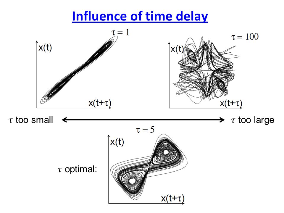
63. Influence of time delay

65. Criterion: Selection of time delay

66. Criterion: Selection of embedding dimension [Kennel & Abarbanel, Phys Rev A 1992]

67. Non-linear measures

68. Non-linear deterministic systems No analytic solution of non-linear differential equations Superposition of solutions not necessarily a solution Behavior of system qualitatively rich e.g. change of dynamics in dependence of control parameter (bifurcations) Sensitive dependence on initial conditions Deterministic chaos

69. Bifurcation diagram: Logistic map Bifurcation: Dynamic change in dependence of control parameter Fixed point Period doublingChaos

70. Deterministic chaos Chaos (every-day use): - State of disorder and irregularity Deterministic chaos - irregular (non-periodic) evolution of state variables - unpredictable (or only short-time predictability) - described by deterministic state equations (in contrast to stochastic systems) - shows instabilities and recurrences

71. Deterministic chaos regularchaoticrandom deterministic stochastic Long-time predictions possible Rather un- predictable unpredictable Strong causalityNo strong causality Non-linearity Uncontrolled (external) influences

72. Characterization of non-linear systems Linear meaures: Static measures (e.g. moments of amplitude distribution): -Some hints on non-linearity -No information about dynamics Dynamic measures (autocorrelation and Fourier spectrum) Autocorrelation Fourier Fast decay, no memory Typically broadband Distinction from noise? Wiener-Khinchin-Theorem

73. Characterizition of a dynamic in phase space Predictability (Information / Entropy) Density Self-similarityLinearity / Non-linearity Determinism / Stochasticity (Dimension) Stability (sensitivity to initial conditions)

74. Lyapunov-exponent

75. Stability

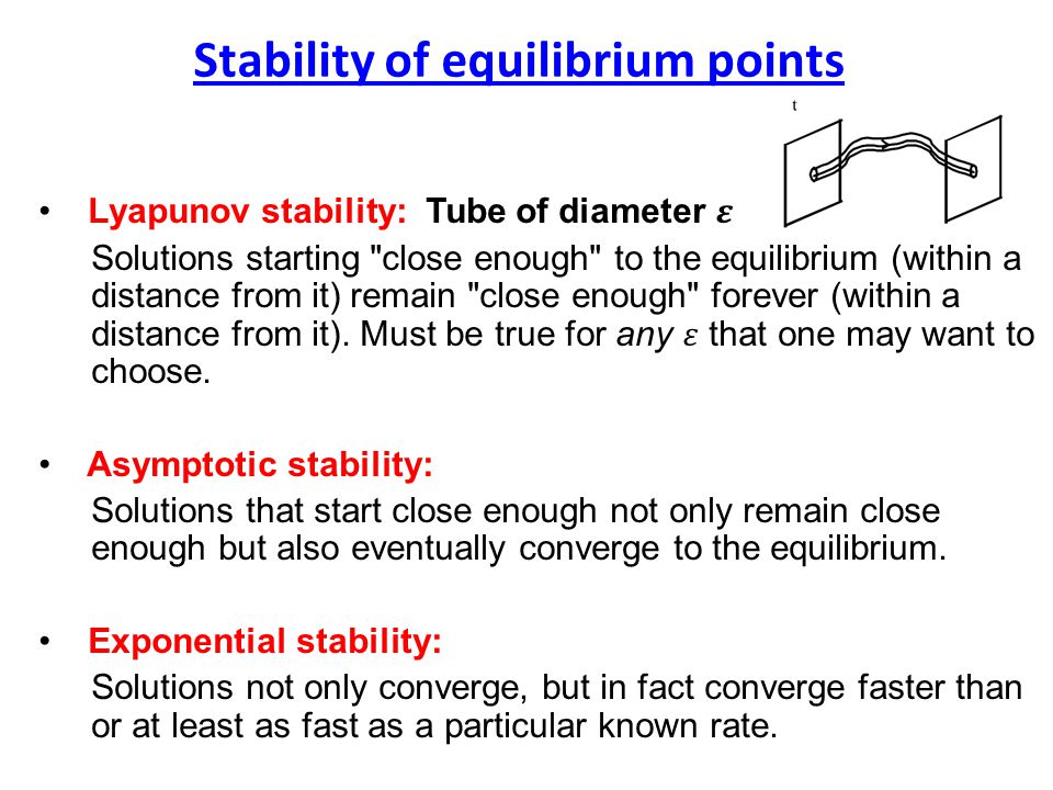
76. Stability of equilibrium points

78. Divergence and convergence Chaotic trajectories are Lyapunov-instable: Divergence: Neighboring trajectories expand Such that their distance increases exponentially (Expansion) Convergence: Expansion of trajectories to the attractor limits is followed by a decrease of distance (Folding).  Sensitive dependence on initial conditions Quantification: Lyapunov-exponent

79. Lyapunov-exponent - Jacobi-Matrix Taylor series - Lyapunov exponent

80. Lyapunov-exponent

81. Example: Logistic map

82. Lyapunov-exponent

83. Largest Lyapunov-exponent: Estimation [Wolf et al. Determining Lyapunov exponents from a time series, Physica D 1985]

84. Non-linear model systems Linear measures Introduction to non-linear dynamics Non-linear measures - Introduction to phase space reconstruction - Lyapunov exponent Today’s lecture

85. Non-linear measures - Dimension - Entropies - Determinism - Tests for Non-linearity, Time series surrogates Next lecture