Download presentation
Presentation is loading. Please wait.

1
Leonardo de Moura Microsoft Research

2
Many approaches Graph-based for difference logic: a – b 3 Fourier-Motzkin elimination: Standard Simplex General Form Simplex

3
Very useful in practice! Most arithmetical constraints in software verification/analysis are in this fragment. x := x + 1 x 1 = x 0 + 1 x 1 - x 0 1, x 0 - x 1 - 1

5
Chasing negative cycles! Algorithms based on Bellman-Ford (O(mn)).
).")
6
Many solvers (e.g., ICS, Simplify) are based on the Standard Simplex. a - d + 2e = 3 b - d = 1 c + d - e = -1 a, b, c, d, e ≥ 0

7
Many solvers (e.g., ICS, Simplify) are based on the Standard Simplex. a - d + 2e = 3 b - d = 1 c + d - e = -1 a, b, c, d, e ≥ 0 1 0 0 -1 2 0 1 0 -1 0 0 0 1 1 -1 abcdeabcde 3 1 =

8
Many solvers (e.g., ICS, Simplify) are based on the Standard Simplex. a - d + 2e = 3 b - d = 1 c + d - e = -1 a, b, c, d, e ≥ 0 1 0 0 -1 2 0 1 0 -1 0 0 0 1 1 -1 abcdeabcde 3 1 = We say a,b,c are the basic (or dependent) variables
 variables.")
9
Many solvers (e.g., ICS, Simplify) are based on the Standard Simplex. a - d + 2e = 3 b - d = 1 c + d - e = -1 a, b, c, d, e ≥ 0 1 0 0 -1 2 0 1 0 -1 0 0 0 1 1 -1 abcdeabcde 3 1 = We say a,b,c are the basic (or dependent) variables We say d,e are the non-basic (or non- dependent) variables. We say d,e are the non-basic (or non- dependent) variables.
 variables We say d,e are the non-basic (or non- dependent) variables. We say d,e are the non-basic (or non- dependent) variables..")
10
Incrementality: add/remove equations Slow backtracking No theory propagation

11
Simplex General Form Algorithm based on the dual simplex Non redundant proofs Efficient backtracking Efficient theory propagation Support for string inequalities: t > 0 Preprocessing step Integer problems: Gomory cuts, Branch & Bound, GCD test

13
s 1 x + y, s 2 x + 2y

14
s 1 = x + y, s 2 = x + 2y

15
s 1 x + y, s 2 x + 2y s 1 = x + y, s 2 = x + 2y s 1 - x - y = 0 s 2 - x - 2y = 0

16
s 1 x + y, s 2 x + 2y s 1 = x + y, s 2 = x + 2y s 1 - x - y = 0 s 2 - x - 2y = 0 s 1, s 2 are basic (dependent) x,y are non-basic
 x,y are non-basic")
17
A way to swap a basic with a non-basic variable! It is just equational reasoning. Key invariant: a basic variable occurs in only one equation. Example: swap s 1 and y s 1 - x - y = 0 s 2 - x - 2y = 0

18
A way to swap a basic with a non-basic variable! It is just equational reasoning. Key invariant: a basic variable occurs in only one equation. Example: swap s 1 and y s 1 - x - y = 0 s 2 - x - 2y = 0 -s 1 + x + y = 0 s 2 - x - 2y = 0

19
A way to swap a basic with a non-basic variable! It is just equational reasoning. Key invariant: a basic variable occurs in only one equation. Example: swap s 1 and y s 1 - x - y = 0 s 2 - x - 2y = 0 -s 1 + x + y = 0 s 2 - x - 2y = 0 -s 1 + x + y = 0 s 2 - 2s 1 + x = 0

20
A way to swap a basic with a non-basic variable! It is just equational reasoning. Key invariant: a basic variable occurs in only one equation. Example: swap s 1 and y s 1 - x - y = 0 s 2 - x - 2y = 0 -s 1 + x + y = 0 s 2 - x - 2y = 0 -s 1 + x + y = 0 s 2 - 2s 1 + x = 0 It is just substituting equals by equals.

21
A way to swap a basic with a non-basic variable! It is just equational reasoning. Key invariant: a basic variable occurs in only one equation. Example: swap s 1 and y s 1 - x - y = 0 s 2 - x - 2y = 0 -s 1 + x + y = 0 s 2 - x - 2y = 0 -s 1 + x + y = 0 s 2 - 2s 1 + x = 0 It is just substituting equals by equals. Definition: An assignment (model) is a mapping from variables to values Definition: An assignment (model) is a mapping from variables to values Key Property: If an assignment satisfies the equations before a pivoting step, then it will also satisfy them after! Key Property: If an assignment satisfies the equations before a pivoting step, then it will also satisfy them after!
 is a mapping from variables to values Definition: An assignment (model) is a mapping from variables to values Key Property: If an assignment satisfies the equations before a pivoting step, then it will also satisfy them after. Key Property: If an assignment satisfies the equations before a pivoting step, then it will also satisfy them after!.")
22
A way to swap a basic with a non-basic variable! It is just equational reasoning. Key invariant: a basic variable occurs in only one equation. Example: swap s 2 and y s 1 - x - y = 0 s 2 - x - 2y = 0 -s 1 + x + y = 0 s 2 - x - 2y = 0 -s 1 + x + y = 0 s 2 - 2s 1 + x = 0 It is just substituting equals by equals. Definition: An assignment (model) is a mapping from variables to values Definition: An assignment (model) is a mapping from variables to values Key Property: If an assignment satisfies the equations before a pivoting step, then it will also satisfy them after! Key Property: If an assignment satisfies the equations before a pivoting step, then it will also satisfy them after! Example: M(x) = 1 M(y) = 1 M(s 1 ) = 2 M(s 2 ) = 3 Example: M(x) = 1 M(y) = 1 M(s 1 ) = 2 M(s 2 ) = 3
 is a mapping from variables to values Definition: An assignment (model) is a mapping from variables to values Key Property: If an assignment satisfies the equations before a pivoting step, then it will also satisfy them after. Key Property: If an assignment satisfies the equations before a pivoting step, then it will also satisfy them after. Example: M(x) = 1 M(y) = 1 M(s 1 ) = 2 M(s 2 ) = 3 Example: M(x) = 1 M(y) = 1 M(s 1 ) = 2 M(s 2 ) = 3.")
24
If the assignment of a non-basic variable does not satisfy a bound, then fix it and propagate the change to all dependent variables. a = c – d b = c + d M(a) = 0 M(b) = 0 M(c) = 0 M(d) = 0 1 c a = c – d b = c + d M(a) = 1 M(b) = 1 M(c) = 1 M(d) = 0 1 c
 = 0 M(b) = 0 M(c) = 0 M(d) = 0 1 c a = c – d b = c + d M(a) = 1 M(b) = 1 M(c) = 1 M(d) = 0 1 c.")
25
If the assignment of a non-basic variable does not satisfy a bound, then fix it and propagate the change to all dependent variables. Of course, we may introduce new “problems”. a = c – d b = c + d M(a) = 0 M(b) = 0 M(c) = 0 M(d) = 0 1 c a 0 a = c – d b = c + d M(a) = 1 M(b) = 1 M(c) = 1 M(d) = 0 1 c a 0
 = 0 M(b) = 0 M(c) = 0 M(d) = 0 1 c a 0 a = c – d b = c + d M(a) = 1 M(b) = 1 M(c) = 1 M(d) = 0 1 c a 0.")
26
If the assignment of a basic variable does not satisfy a bound, then pivot it, fix it, and propagate the change to its new dependent variables. a = c – d b = c + d M(a) = 0 M(b) = 0 M(c) = 0 M(d) = 0 1 a c = a + d b = a + 2d M(a) = 0 M(b) = 0 M(c) = 0 M(d) = 0 1 a c = a + d b = a + 2d M(a) = 1 M(b) = 1 M(c) = 1 M(d) = 0 1 a
 = 0 M(b) = 0 M(c) = 0 M(d) = 0 1 a c = a + d b = a + 2d M(a) = 0 M(b) = 0 M(c) = 0 M(d) = 0 1 a c = a + d b = a + 2d M(a) = 1 M(b) = 1 M(c) = 1 M(d) = 0 1 a.")
27
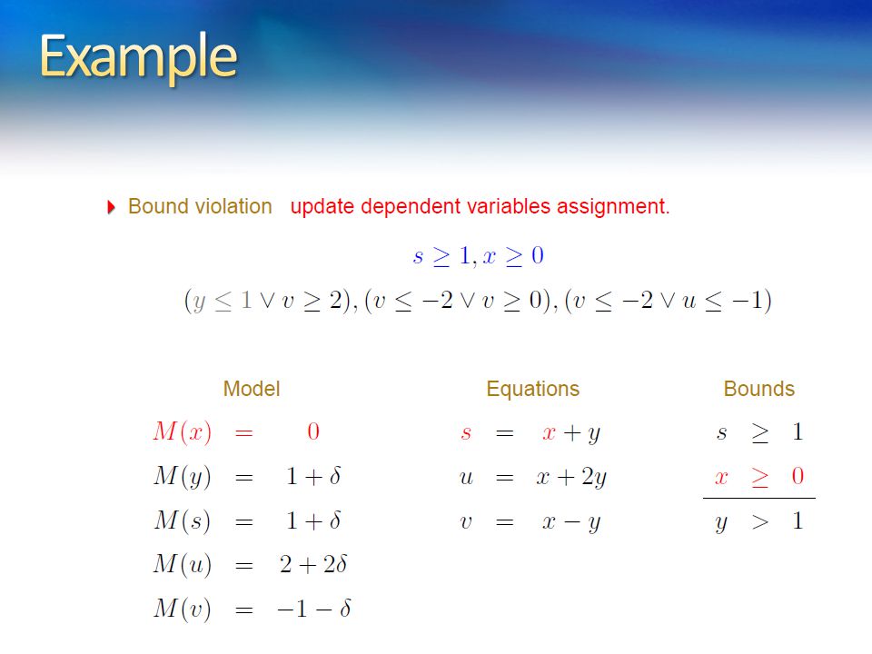
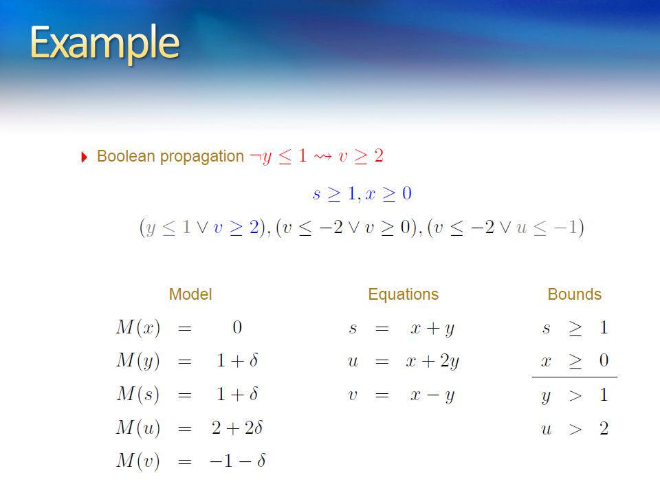
Sometimes, a model cannot be repaired. It is pointless to pivot. a = b – c a 0, 1 b, c 0 M(a) = 1 M(b) = 1 M(c) = 0 The value of M(a) is too big. We can reduce it by: - reducing M(b) not possible b is at lower bound - increasing M(c) not possible c is at upper bound The value of M(a) is too big. We can reduce it by: - reducing M(b) not possible b is at lower bound - increasing M(c) not possible c is at upper bound
 = 1 M(b) = 1 M(c) = 0 The value of M(a) is too big. We can reduce it by: - reducing M(b) not possible b is at lower bound - increasing M(c) not possible c is at upper bound The value of M(a) is too big. We can reduce it by: - reducing M(b) not possible b is at lower bound - increasing M(c) not possible c is at upper bound.")
28
s 1 a + d, s 2 c + d a = s 1 – s 2 + c a 0, 1 s 1, s 2 0, 0 c M(a) = 1 M(s 1 ) = 1 M(s 2 ) = 0 M(c) = 0 Extracting proof from failed repair attempts is easy.
 = 1 M(s 1 ) = 1 M(s 2 ) = 0 M(c) = 0 Extracting proof from failed repair attempts is easy.")
29
s 1 a + d, s 2 c + d a = s 1 – s 2 + c a 0, 1 s 1, s 2 0, 0 c M(a) = 1 M(s 1 ) = 1 M(s 2 ) = 0 M(c) = 0 Extracting proof from failed repair attempts is easy. { a 0, 1 s 1, s 2 0, 0 c } is inconsistent

30
s 1 a + d, s 2 c + d a = s 1 – s 2 + c a 0, 1 s 1, s 2 0, 0 c M(a) = 1 M(s 1 ) = 1 M(s 2 ) = 0 M(c) = 0 Extracting proof from failed repair attempts is easy. { a 0, 1 s 1, s 2 0, 0 c } is inconsistent { a 0, 1 a + d, c + d 0, 0 c } is inconsistent

32
SMT@Microsoft

85
Completeness: trivial Soundness: also trivial Termination: non trivial. We cannot choose arbitrary variable to pivot. Assume the variables are ordered. Bland’s rule: select the smallest basic variable c that does not satisfy its bounds, then select the smallest non-basic in the row of c that can be used for pivoting. Too technical. Uses the fact that a tableau has a finite number of configurations. Then, any infinite trace will have cycles.

86
Array of rows (equations). Each row is a dynamic array of tuples: (coefficient, variable, pos_in_occs, is_dead) Each variable x has a “set” (dynamic array) of occurrences: (row_idx, pos_in_row, is_dead) Each variable x has a “field” row[x] row[x] is -1 if x is non basic otherwise, row[x] contains the idx of the row containing x Each variable x has “fields”: lower[x], upper[x], and value[x]
 Each variable x has a set (dynamic array) of occurrences: (row_idx, pos_in_row, is_dead) Each variable x has a field row[x] row[x] is -1 if x is non basic otherwise, row[x] contains the idx of the row containing x Each variable x has fields : lower[x], upper[x], and value[x].")
87
rows: array of rows (equations). Each row is a dynamic array of tuples: (coefficient, variable, pos_in_occs, is_dead) occs[x]: Each variable x has a “set” (dynamic array) of occurrences: (row_idx, pos_in_row, is_dead) row[x]: row[x] is -1 if x is non basic otherwise, row[x] contains the idx of the row containing x Other “fields”: lower[x], upper[x], and value[x] atoms[x]: atoms (assigned/unassigned) that contains x
 occs[x]: Each variable x has a set (dynamic array) of occurrences: (row_idx, pos_in_row, is_dead) row[x]: row[x] is -1 if x is non basic otherwise, row[x] contains the idx of the row containing x Other fields : lower[x], upper[x], and value[x] atoms[x]: atoms (assigned/unassigned) that contains x.")
88
s 1 a + b, s 2 c – b p 1 a 0, p 2 1 s 1, p 3 1 s 2 p 1, p 2 were already assigned a - s 1 + s 2 + c = 0 b- c + s 2 = 0 a 0, 1 s 1 M(a) = 0 value[a] = 0 M(b) = -1 value[a] = -1 M(c) = 0 value[c] = 0 M(s 1 ) = 1 value[s 1 ] = 1 M(s 2 ) = 1 value[s 2 ] = 1 rows = [ [(1, a, 0, t), (-1, s 1, 0, t), (1, s 2, 1, t), (1, c, 0, t)], [(1,b, 0, t), (-1, c, 1, t), (1, s 2, 2, t)] ] occs[a] = [(0, 0, f)] occs[b] = [(1,0,f)] occs[c] = [(0,3,f), (1,1,f)] occs[s 1 ] = [(0,1,f)] occs[s 2 ] = [(0,0,t), (0,2,f), (1,2,f)] row[a] = 0, row[b] = 1, row[c] = -1, … upper[a] = 0, lower[s 1 ] = 1 atoms[a] = {p 1 }, atoms[s 1 ] = {p 2 }, …
![s 1 a + b, s 2 c – b p 1 a 0, p 2 1 s 1, p 3 1 s 2 p 1, p 2 were already assigned a - s 1 + s 2 + c = 0 b- c + s 2 = 0 a 0, 1 s 1 M(a) = 0 value[a] = 0 M(b) = -1 value[a] = -1 M(c) = 0 value[c] = 0 M(s 1 ) = 1 value[s 1 ] = 1 M(s 2 ) = 1 value[s 2 ] = 1 rows = [ [(1, a, 0, t), (-1, s 1, 0, t), (1, s 2, 1, t), (1, c, 0, t)], [(1,b, 0, t), (-1, c, 1, t), (1, s 2, 2, t)] ] occs[a] = [(0, 0, f)] occs[b] = [(1,0,f)] occs[c] = [(0,3,f), (1,1,f)] occs[s 1 ] = [(0,1,f)] occs[s 2 ] = [(0,0,t), (0,2,f), (1,2,f)] row[a] = 0, row[b] = 1, row[c] = -1, … upper[a] = 0, lower[s 1 ] = 1 atoms[a] = {p 1 }, atoms[s 1 ] = {p 2 }, …](http://images.slideplayer.com/20/5929482/slides/slide_88.jpg "s 1 a + b, s 2 c – b p 1 a 0, p 2 1 s 1, p 3 1 s 2 p 1, p 2 were already assigned a - s 1 + s 2 + c = 0 b- c + s 2 = 0 a 0, 1 s 1 M(a) = 0 value[a] = 0 M(b) = -1 value[a] = -1 M(c) = 0 value[c] = 0 M(s 1 ) = 1 value[s 1 ] = 1 M(s 2 ) = 1 value[s 2 ] = 1 rows = [ [(1, a, 0, t), (-1, s 1, 0, t), (1, s 2, 1, t), (1, c, 0, t)], [(1,b, 0, t), (-1, c, 1, t), (1, s 2, 2, t)] ] occs[a] = [(0, 0, f)] occs[b] = [(1,0,f)] occs[c] = [(0,3,f), (1,1,f)] occs[s 1 ] = [(0,1,f)] occs[s 2 ] = [(0,0,t), (0,2,f), (1,2,f)] row[a] = 0, row[b] = 1, row[c] = -1, … upper[a] = 0, lower[s 1 ] = 1 atoms[a] = {p 1 }, atoms[s 1 ] = {p 2 }, …")
89
In practice, we need a combination of theories. b + 2 = c and f(read(write(a,b,3), c-2)) ≠ f(c-b+1) A theory is a set (potentially infinite) of first-order sentences. Main questions: Is the union of two theories T1 T2 consistent? Given a solvers for T1 and T2, how can we build a solver for T1 T2?
, c-2)) ≠ f(c-b+1) A theory is a set (potentially infinite) of first-order sentences. Main questions: Is the union of two theories T1 T2 consistent. Given a solvers for T1 and T2, how can we build a solver for T1 T2 .")
90
Two theories are disjoint if they do not share function/constant and predicate symbols. = is the only exception. Example: The theories of arithmetic and arrays are disjoint. Arithmetic symbols: {0, -1, 1, -2, 2, …, +, -, *, >, <, ≥, } Array symbols: { read, write }

91
It is a different name for our “naming” subterms procedure. b + 2 = c, f(read(write(a,b,3), c-2)) ≠ f(c-b+1) b + 2 = c, v 6 ≠ v 7 v 1 3, v 2 write(a, b, v 1 ), v 3 c-2, v 4 read(v 2, v 3 ), v 5 c-b+1, v 6 f(v 4 ), v 7 f(v 5 )
, c-2)) ≠ f(c-b+1) b + 2 = c, v 6 ≠ v 7 v 1 3, v 2 write(a, b, v 1 ), v 3 c-2, v 4 read(v 2, v 3 ), v 5 c-b+1, v 6 f(v 4 ), v 7 f(v 5 ).")
92
It is a different name for our “naming” subterms procedure. b + 2 = c, f(read(write(a,b,3), c-2)) ≠ f(c-b+1) b + 2 = c, v 6 ≠ v 7 v 1 3, v 2 write(a, b, v 1 ), v 3 c-2, v 4 read(v 2, v 3 ), v 5 c-b+1, v 6 f(v 4 ), v 7 f(v 5 ) b + 2 = c, v 1 3, v 3 c-2, v 5 c-b+1, v 2 write(a, b, v 1 ), v 4 read(v 2, v 3 ), v 6 f(v 4 ), v 7 f(v 5 ), v 6 ≠ v 7
, c-2)) ≠ f(c-b+1) b + 2 = c, v 6 ≠ v 7 v 1 3, v 2 write(a, b, v 1 ), v 3 c-2, v 4 read(v 2, v 3 ), v 5 c-b+1, v 6 f(v 4 ), v 7 f(v 5 ) b + 2 = c, v 1 3, v 3 c-2, v 5 c-b+1, v 2 write(a, b, v 1 ), v 4 read(v 2, v 3 ), v 6 f(v 4 ), v 7 f(v 5 ), v 6 ≠ v 7.")
93
A theory is stably infinite if every satisfiable QFF is satisfiable in an infinite model. EUF and arithmetic are stably infinite. Bit-vectors are not.

94
The union of two consistent, disjoint, stably infinite theories is consistent.

95
A theory T is convex iff for all finite sets S of literals and for all a 1 = b 1 … a n = b n S implies a 1 = b 1 … a n = b n iff S implies a i = b i for some 1 i n

96
Every convex theory with non trivial models is stably infinite. All Horn equational theories are convex. formulas of the form s 1 ≠ r 1 … s n ≠ r n t = t’ Linear rational arithmetic is convex.

97
Linear integer arithmetic is not convex 1 a 2, b = 1, c = 2 implies a = b a = c Nonlinear arithmetic a 2 = 1, b = 1, c = -1 implies a = b a = c Theory of bit-vectors Theory of arrays c 1 = read(write(a, i, c 2 ), j), c 3 = read(a, j) implies c 1 = c 2 c 1 = c 3
, j), c 3 = read(a, j) implies c 1 = c 2 c 1 = c 3")
98
EUF is convex (O(n log n)) IDL is non-convex (O(nm)) EUF IDL is NP-Complete Reduce 3CNF to EUF IDL For each boolean variable p i add 0 a i 1 For each clause p 1 p 2 p 3 add f(a 1, a 2, a 3 ) ≠ f(0, 1, 0)
) IDL is non-convex (O(nm)) EUF IDL is NP-Complete Reduce 3CNF to EUF IDL For each boolean variable p i add 0 a i 1 For each clause p 1 p 2 p 3 add f(a 1, a 2, a 3 ) ≠ f(0, 1, 0)")
99
EUF is convex (O(n log n)) IDL is non-convex (O(nm)) EUF IDL is NP-Complete Reduce 3CNF to EUF IDL For each boolean variable p i add 0 a i 1 For each clause p 1 p 2 p 3 add f(a 1, a 2, a 3 ) ≠ f(0, 1, 0) a 1 ≠ 0 a 2 ≠ 1 a 3 ≠ 0 implies
) IDL is non-convex (O(nm)) EUF IDL is NP-Complete Reduce 3CNF to EUF IDL For each boolean variable p i add 0 a i 1 For each clause p 1 p 2 p 3 add f(a 1, a 2, a 3 ) ≠ f(0, 1, 0) a 1 ≠ 0 a 2 ≠ 1 a 3 ≠ 0 implies")
106
b + 2 = c, f(read(write(a,b,3), c-2)) ≠ f(c-b+1) Arithmetic b + 2 = c, v 1 3, v 3 c-2, v 5 c-b+1 Arrays v 2 write(a, b, v 1 ), v 4 read(v 2, v 3 ) EUF v 6 f(v 4 ), v 7 f(v 5 ), v 6 ≠ v 7
, c-2)) ≠ f(c-b+1) Arithmetic b + 2 = c, v 1 3, v 3 c-2, v 5 c-b+1 Arrays v 2 write(a, b, v 1 ), v 4 read(v 2, v 3 ) EUF v 6 f(v 4 ), v 7 f(v 5 ), v 6 ≠ v 7")
107
b + 2 = c, f(read(write(a,b,3), c-2)) ≠ f(c-b+1) Arithmetic b + 2 = c, v 1 3, v 3 c-2, v 5 c-b+1 Arrays v 2 write(a, b, v 1 ), v 4 read(v 2, v 3 ) EUF v 6 f(v 4 ), v 7 f(v 5 ), v 6 ≠ v 7 Substituting c
, c-2)) ≠ f(c-b+1) Arithmetic b + 2 = c, v 1 3, v 3 c-2, v 5 c-b+1 Arrays v 2 write(a, b, v 1 ), v 4 read(v 2, v 3 ) EUF v 6 f(v 4 ), v 7 f(v 5 ), v 6 ≠ v 7 Substituting c")
108
b + 2 = c, f(read(write(a,b,3), c-2)) ≠ f(c-b+1) Arithmetic b + 2 = c, v 1 3, v 3 b, v 5 3 Arrays v 2 write(a, b, v 1 ), v 4 read(v 2, v 3 ), EUF v 6 f(v 4 ), v 7 f(v 5 ), v 6 ≠ v 7 Propagating v 3 = b
, c-2)) ≠ f(c-b+1) Arithmetic b + 2 = c, v 1 3, v 3 b, v 5 3 Arrays v 2 write(a, b, v 1 ), v 4 read(v 2, v 3 ), EUF v 6 f(v 4 ), v 7 f(v 5 ), v 6 ≠ v 7 Propagating v 3 = b")
109
b + 2 = c, f(read(write(a,b,3), c-2)) ≠ f(c-b+1) Arithmetic b + 2 = c, v 1 3, v 3 b, v 5 3 Arrays v 2 write(a, b, v 1 ), v 4 read(v 2, v 3 ), v 3 = b EUF v 6 f(v 4 ), v 7 f(v 5 ), v 6 ≠ v 7, v 3 = b Deducing v 4 = v 1
, c-2)) ≠ f(c-b+1) Arithmetic b + 2 = c, v 1 3, v 3 b, v 5 3 Arrays v 2 write(a, b, v 1 ), v 4 read(v 2, v 3 ), v 3 = b EUF v 6 f(v 4 ), v 7 f(v 5 ), v 6 ≠ v 7, v 3 = b Deducing v 4 = v 1")
110
b + 2 = c, f(read(write(a,b,3), c-2)) ≠ f(c-b+1) Arithmetic b + 2 = c, v 1 3, v 3 b, v 5 3 Arrays v 2 write(a, b, v 1 ), v 4 read(v 2, v 3 ), v 3 = b, v 4 = v 1 EUF v 6 f(v 4 ), v 7 f(v 5 ), v 6 ≠ v 7, v 3 = b Propagating v 4 = v 1
, c-2)) ≠ f(c-b+1) Arithmetic b + 2 = c, v 1 3, v 3 b, v 5 3 Arrays v 2 write(a, b, v 1 ), v 4 read(v 2, v 3 ), v 3 = b, v 4 = v 1 EUF v 6 f(v 4 ), v 7 f(v 5 ), v 6 ≠ v 7, v 3 = b Propagating v 4 = v 1")
111
b + 2 = c, f(read(write(a,b,3), c-2)) ≠ f(c-b+1) Arithmetic b + 2 = c, v 1 3, v 3 b, v 5 3, v 4 = v 1 Arrays v 2 write(a, b, v 1 ), v 4 read(v 2, v 3 ), v 3 = b, v 4 = v 1 EUF v 6 f(v 4 ), v 7 f(v 5 ), v 6 ≠ v 7, v 3 = b, v 4 = v 1 Propagating v 5 = v 1
, c-2)) ≠ f(c-b+1) Arithmetic b + 2 = c, v 1 3, v 3 b, v 5 3, v 4 = v 1 Arrays v 2 write(a, b, v 1 ), v 4 read(v 2, v 3 ), v 3 = b, v 4 = v 1 EUF v 6 f(v 4 ), v 7 f(v 5 ), v 6 ≠ v 7, v 3 = b, v 4 = v 1 Propagating v 5 = v 1")
112
b + 2 = c, f(read(write(a,b,3), c-2)) ≠ f(c-b+1) Arithmetic b + 2 = c, v 1 3, v 3 b, v 5 3, v 4 = v 1 Arrays v 2 write(a, b, v 1 ), v 4 read(v 2, v 3 ), v 3 = b, v 4 = v 1 EUF v 6 f(v 4 ), v 7 f(v 5 ), v 6 ≠ v 7, v 3 = b, v 4 = v 1, v 5 = v 1 Congruence: v 6 = v 7
, c-2)) ≠ f(c-b+1) Arithmetic b + 2 = c, v 1 3, v 3 b, v 5 3, v 4 = v 1 Arrays v 2 write(a, b, v 1 ), v 4 read(v 2, v 3 ), v 3 = b, v 4 = v 1 EUF v 6 f(v 4 ), v 7 f(v 5 ), v 6 ≠ v 7, v 3 = b, v 4 = v 1, v 5 = v 1 Congruence: v 6 = v 7")
113
b + 2 = c, f(read(write(a,b,3), c-2)) ≠ f(c-b+1) Arithmetic b + 2 = c, v 1 3, v 3 b, v 5 3, v 4 = v 1 Arrays v 2 write(a, b, v 1 ), v 4 read(v 2, v 3 ), v 3 = b, v 4 = v 1 EUF v 6 f(v 4 ), v 7 f(v 5 ), v 6 ≠ v 7, v 3 = b, v 4 = v 1, v 5 = v 1, v 6 = v 7 Unsatisfiable
, c-2)) ≠ f(c-b+1) Arithmetic b + 2 = c, v 1 3, v 3 b, v 5 3, v 4 = v 1 Arrays v 2 write(a, b, v 1 ), v 4 read(v 2, v 3 ), v 3 = b, v 4 = v 1 EUF v 6 f(v 4 ), v 7 f(v 5 ), v 6 ≠ v 7, v 3 = b, v 4 = v 1, v 5 = v 1, v 6 = v 7 Unsatisfiable")
114
Deterministic procedure may fail for non-convex theories. 0 a 1, 0 b 1, 0 c 1, f(a) ≠ f(b), f(a) ≠ f(c), f(b) ≠ f(c)
 ≠ f(b), f(a) ≠ f(c), f(b) ≠ f(c).")
127
Model mutation without pivoting For each non basic variable x j compute [L j, U j ] Each row containing x j enforces a limit on how much it can be increase and/or decreased without violating the bounds of the basic variable in the row.
![Model mutation without pivoting For each non basic variable x j compute [L j, U j ] Each row containing x j enforces a limit on how much it can be increase and/or decreased without violating the bounds of the basic variable in the row.](http://images.slideplayer.com/20/5929482/slides/slide_127.jpg "Model mutation without pivoting For each non basic variable x j compute [L j, U j ] Each row containing x j enforces a limit on how much it can be increase and/or decreased without violating the bounds of the basic variable in the row.")
128
We say a variable is fixed if the lower and upper bound are the same. 1 x 1 A polynomial P is fixed if all its variables are fixed. Given a fixed polynomial P of the forma 2x 1 + x 2, we use M(P) to denote 2M(x 1 ) + M(x 2 )
 to denote 2M(x 1 ) + M(x 2 ).")
129
M MM MM

131
A reduction function reduces the satifiability problem for a complex theory into the satisfiability problem of a simpler theory. Ackermannization is a reduction function.

132
EUF

Similar presentations


 Literal: propositional variable or its negation p >")
 Computer Science cpsc422, Lecture 21 Mar, 4, 2015 Slide credit: some slides adapted from Stuart.>")


 Interpretation search ( ² ) Quantifiers Equality Decision procedures Induction Cross-cutting aspectsMain search.>")


>")