1. Business Forecasting Chapter 4 Data Collection and Analysis in Forecasting

2. Chapter Topics Preliminary Adjustments to Data Data Transformation Patterns in Time Series Data The Classical Decomposition Method

3. Preliminary Data Adjustments Trading Day Adjustments Price Change Adjustments Population Change Adjustments

4. Trading Day Adjustments Yr JFMAMJJASOND 05 2120232122 2123222122 06 222023202322212322 21 07 232022212321222320232221

5. Trading Day Adjustment Number of Computers Sold (in Millions) in 2005, 2006, and 2007 Month2005 20062007 January345 February445 March356 April536 May536 June547 July656 August646 September657 October554 November564 December665 Yearly unit sales595467

6. Trading Day Adjustment

7. Trading Day Adjustments

8. Price Change Adjustments

9. Having computed the price index, we are now able to deflate the sales revenue with the weighted price index in the following way:

10. Price Change Adjustments To see the impact of separating the effect of price level changes, we graph the price of computers in constant and current dollars.

11. Population Change Adjustments Disposable Personal Income and Per Capita Income for the U.S. 1990 and 2005 Disposable IncomePopulationPer Capita Disposable YearBillions of Dollars(in Millions)Income ($)

12. Data Transformation Most appropriate remedial measure for variance heterogeneity. Original data are converted into a new scale, resulting in a new data set that is expected to satisfy the condition of homogeneity of variance. Several transformation techniques are available.

13. Data Transformation Linear Transformation: An important assumption in using the regression model for forecasting is that the pattern of observation is linear. Obviously, there are many situations in which this is not a valid assumption. For example, if we were forecasting monthly sales and it was believed that those sales varied according to the season of the year, then the assumption of linearity would not hold.

14. Linear Transformation A forecasting equation may be of the form: The above could easily be transformed into a linear form for estimation purposes:

15. Logarithmic Transformation

16. Time Operating Revenue 0 2,000 4,000 6,000 8,000 10,000 19881990199219941996199820002002200420062008 1.00 10.00 Log of Operating Revenue ActualLog Figure 4.2 Actual and Logarithmically Transformed Operating Revenue for Southwest Airlines

17. Square Root Transformation

18. Square Root Transformation ( Scaled Square Root Data ) 0 2,000 4,000 6,000 8,000 10,000 19881990199219941996199820002002200420062008 Time 0.00 20.00 40.00 60.00 80.00 100.00 120.00 Operating RevenueSquare Root Operating Revenue

19. Square Root Transformation ( Unscaled Square Root Data )

20. Classical Time Series Model Secular Trend (T ) Seasonal Variation (S ) Cyclical Variation (C ) Random or Irregular Variation

21. Trend Linear Trend Non-linear Trend

22. Trend Computing the Linear Trend The Freehand Method The Semi-average Method The Least Squares Method

23. Freehand Method

24. Since a linear trend by this method is simply an approximation of a straight line equation, we have to determine the intercept and the slope of the line. Based on our data, we have:

25. Freehand Method

26. Now we can use this equation to make a forecast of the trend. For example, the forecast for 2006 would be:

27. Freehand Method Based on your understanding, what are the pitfalls of using the freehand method? Simple method but not objective. Why not objective?

28. The Semi-average Method Simple but objective method in fitting a trend line. Divides the data into two equal parts and computes the average for each part. The computed averages for each part provide two points on a straight line. The slope of the line is computed by taking the difference between the averages and dividing it by half of the total number of observations.

29. The Semi-average Method Fitting a Straight Line by the Semi-Average Method to Income from the Export of Durable Goods, 1996–2005 YearIncomeSemi-totalSemi-averageCoded Time 1996 394.9 −2 1997 466.2−1 1998 481.22,415.1483.02 0 1999 503.6 1 2000 569.2 2 2001 522.2 3 2002 491.2 4 2003 499.82,679535.8 5 2004 556.1 6 2005 609.7

30. The Semi-average Method We see that the intercept of the line is: 483.02 The fitted equation is: The slope is:

31. The Semi-average Method For the year 2005, the forecast revenue from export of durable goods is:

32. The Least Squares Method Provides the best method of fitting a trend. The intercept and the slope are computed as follows:

33. The Least Squares Method Using the data from the previous example, we have:

34. The Least Squares Method The fitted trend line equation is: Note: Since x is measured in a half year, we have to multiply it by two to get the full year. x = 0 in 2000 ½ 1 x = ½ year Y = Billions of Dollars

35. The Least Squares Method To compare the two methods, we note: Least squares: Semi-average:

36. Nonlinear Trend In many business and economic environments we observe that the time series does not follow a constant rate of increase or decrease, but follows an increasing or decreasing pattern. Whenever there is dramatic change in production technology, we expect the trend line not to follow a constant linear pattern.

37. Nonlinear Trend A polynomial function best exemplifies business conditions. A second-degree parabola provides a good historical description of an increase or decrease per time period.

38. Nonlinear Trend To solve for the constants a, b, and c in the previous equation, we use the following simultaneous equations:

39. Nonlinear Trend World Carbon Emissions from Fossil Fuel Burning 1982–1994 YearMillion tonnes 19824,960−6−29,760178,560361,296 19834,947−5−24,735123,67525625 19845,109−4−20,436 81,74416256 19855,282−3−15,846 47,538981 19865,464−2−10,928 21,856416 19875,584−1−5,584 5,58411 19885,801 0 0 000 19895,912 1 5,912 5,92111 19905,941 211,882 23,764416 19916,026 318,078 54,234981 19925,910 423,640 94,56016256 19935,893 529,465147,32525625 19945,925 635,550213,300361,296 72,754 017,238998,0611824,550 XYxxY

40. Nonlinear Trend The data from the table is used to compute the following: x = 0 in 1988 1x = one year Y = million tonnes

41. Logarithmic Trend When we wish to fit a trend line to percentage rates of change, we use the logarithmic trend line. This is more prevalent when dealing with economic growth in an environment. The logarithmic trend equation is:

42. Logarithmic Trend The least squares trend is computed as:

43. Logarithmic Trend Example 1990 620.92.793 − 15 − 41.89225 1991 719.12.857 − 13 − 37.13169 1992 849.42.929 − 11 − 32.22121 1993 917.42.963 − 9 − 26.6681 19941,210.13.083 − 7 − 21.5749 19951,487.83.173 − 5 − 15.8625 19961,510.53.179 − 3 − 9.539 19971,827.93.262 − 1 − 3.261 19981,837.13.26413.261 19991,949.33.29039.869 20002,492.03.397516.9825 20012,661.03.425723.9749 20023,256.03.513931.6181 20034,382.283.6421140.05121 20045,933.23.7731349.05169 20057,619.53.8821558.22225 52.420.0044.89 1360.0 Chinese Exports Year ( $ 100 Million)log Yxx log Y

44. Logarithmic Trend Example (continued)

45. The estimated trend line equation is:

46. Logarithmic Trend (continued) Check the goodness of fit by substituting two data points such as 1992 and 2003, into the fitted equation. For 1992, we will have:

47. Logarithmic Trend (continued) For 2003, we will have:

48. Logarithmic Trend Interpretation of the estimated trend line would be similar to a linear trend. However, before we can interpret the estimated values, we have to convert the log values into actual values of the data points. This is done by taking the antilog.

49. Logarithmic Trend The results are: And

50. Logarithmic Trend To determine the rate of change or the slope of the line we have: R = antilog 0.033 = 1.079 Since the rate of change (r) was defined as R −1, then r = 1.079 −1 = 0.079 r = 7.9 percent per half-year Therefore the growth rate is 15.8% or 16% per year.

51. Other Approaches to Trend Line Two more sophisticated methods of determining whether there is a trend in the data: Differencing Autocorrelation (Box–Jenkins Methodology) Allows the analyst to see whether a linear equation, a second-degree polynomial, or a higher-degree equation should be used to determine a trend.

52. Differencing First Difference Second Difference

53. Differencing Method Example First and Second Difference of Hypothetical Data YtFirst DifferenceSecond Difference 20,000 22,000 2,000 24,300 2,300300 26,900 2,600300 29,800 2,900300 33,000 3,200300

54. Seasonal Analysis Seasonal variation is defined as a predictable and repetitive movement observed around a trend line within a period of 1 year or less. There are several reasons for measuring seasonal variations. When analyzing the data from a time series, it is important to be able to know how much of the variation in the data is due to the seasonal factors.

55. Seasonal Variation (Continued) We may use seasonal variation patterns in making projections or forecasts of a short- term nature. By eliminating the seasonal variation from a time series, we may discover the cyclical pattern of the time series.

56. Seasonal Variation Computation of Ratio of Original Data to Moving Average

57. Seasonal Variation To compute a seasonal index, we do the following: sum the modified means

58. Seasonal Variation

59. If production is full, we expect the index to equal 100 for each month. If not, we have to adjust it by computing a correction factor. Compute the seasonal index.

60. Seasonal Variation

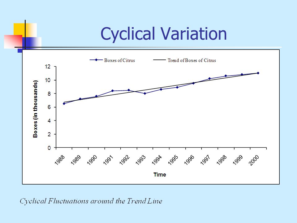
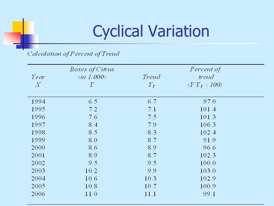
61. Cyclical Variation Similar to seasonal variation except that it occurs every 5 to 10 years. There is a systematic pattern in the data that mirrors what is happening in the economy. Movements from a recession to a depression or recession to recovery follow a cycle. Every time series data has a random component. If there were no random components, we would have perfect prediction of future values. However, this is not the case with real-world conditions. The cyclical component is measured as a proportion of the trend.

62. Cyclical Variation

65. Cyclical Variation Example

66. Chapter Summary Preliminary Adjustments to Data: Trading Day Adjustment Price Adjustment Population Adjustment Data Transformation Patterns in Time Series Data The Classical Decomposition Method