Download presentation
Presentation is loading. Please wait.

1
Centrality in Social Networks Background: At the individual level, one dimension of position in the network can be captured through centrality. Conceptually, centrality is fairly straight forward: we want to identify which nodes are in the ‘center’ of the network. In practice, identifying exactly what we mean by ‘center’ is somewhat complicated. Approaches: Degree Closeness Betweenness Information & Power Graph Level measures: Centralization Applications: (Day 2) Friedkin: Interpersonal Influence in Groups Alderson and Beckfield: World City Systems
 Friedkin: Interpersonal Influence in Groups Alderson and Beckfield: World City Systems.")
2
Centrality in Social Networks Centrality and Network Flow

3
In recent work, Borgatti (2003; 2005) discusses centrality in terms of two key dimensions: Radial Medial Frequency Distance Degree Centrality Bon. Power centrality Closeness Centrality Betweenness (empty: but would be an interruption measure based on distance, but see Borgatti forthcoming) Centrality in Social Networks Power / Eigenvalue
 Centrality in Social Networks Power / Eigenvalue.")
4
He expands this set in the paper w. Everet to look at the “production” side. -All measures are features of a nodes position in the pattern of “walks” on networks: -Walk Type (geodesic, edge-disjoint) -Walk Property (i.e Volume, length) -Walk Position (Node involvement – radial, medial – passing through or ending on, etc.) -Summary type (Sum, mean, etc.) Centrality in Social Networks Power / Eigenvalue Ultimately dyadic cohesion of sundry sorts is the thing being summarized
 -Walk Property (i.e Volume, length) -Walk Position (Node involvement – radial, medial – passing through or ending on, etc.) -Summary type (Sum, mean, etc.) Centrality in Social Networks Power / Eigenvalue Ultimately dyadic cohesion of sundry sorts is the thing being summarized.")
5
Intuitively, we want a method that allows us to distinguish “important” actors. Consider the following graphs: Centrality in Social Networks

6
The most intuitive notion of centrality focuses on degree: The actor with the most ties is the most important: Centrality in Social Networks Degree

7
In a simple random graph (G n,p ), degree will have a Poisson distribution, and the nodes with high degree are likely to be at the intuitive center. Deviations from a Poisson distribution suggest non-random processes, which is at the heart of current “scale-free” work on networks (see below). Centrality in Social Networks Degree
. Centrality in Social Networks Degree.")
8
Degree centrality, however, can be deceiving, because it is a purely local measure. Centrality in Social Networks Degree

9
If we want to measure the degree to which the graph as a whole is centralized, we look at the dispersion of centrality: Simple: variance of the individual centrality scores. Or, using Freeman’s general formula for centralization (which ranges from 0 to 1): UCINET, SPAN, PAJEK and most other network software will calculate these measures. Centrality in Social Networks Degree
: UCINET, SPAN, PAJEK and most other network software will calculate these measures. Centrality in Social Networks Degree.")
10
Degree Centralization Scores Freeman:.07 Variance:.20 Freeman: 1.0 Variance: 3.9 Freeman:.02 Variance:.17 Freeman: 0.0 Variance: 0.0 Centrality in Social Networks Degree

11
A second measure of centrality is closeness centrality. An actor is considered important if he/she is relatively close to all other actors. Closeness is based on the inverse of the distance of each actor to every other actor in the network. Closeness Centrality: Normalized Closeness Centrality Centrality in Social Networks Closeness

12
Distance Closeness normalized 0 1 1 1 1 1 1 1.143 1.00 1 0 2 2 2 2 2 2.077.538 1 2 0 2 2 2 2 2.077.538 1 2 2 0 2 2 2 2.077.538 1 2 2 2 0 2 2 2.077.538 1 2 2 2 2 0 2 2.077.538 1 2 2 2 2 2 0 2.077.538 1 2 2 2 2 2 2 0.077.538 Closeness Centrality in the examples Distance Closeness normalized 0 1 2 3 4 4 3 2 1.050.400 1 0 1 2 3 4 4 3 2.050.400 2 1 0 1 2 3 4 4 3.050.400 3 2 1 0 1 2 3 4 4.050.400 4 3 2 1 0 1 2 3 4.050.400 4 4 3 2 1 0 1 2 3.050.400 3 4 4 3 2 1 0 1 2.050.400 2 3 4 4 3 2 1 0 1.050.400 1 2 3 4 4 3 2 1 0.050.400 Centrality in Social Networks Closeness

13
Distance Closeness normalized 0 1 2 3 4 5 6.048.286 1 0 1 2 3 4 5.063.375 2 1 0 1 2 3 4.077.462 3 2 1 0 1 2 3.083.500 4 3 2 1 0 1 2.077.462 5 4 3 2 1 0 1.063.375 6 5 4 3 2 1 0.048.286 Closeness Centrality in the examples Centrality in Social Networks Degree

14
Distance Closeness normalized 0 1 1 2 3 4 4 5 5 6 5 5 6.021.255 1 0 1 1 2 3 3 4 4 5 4 4 5.027.324 1 1 0 1 2 3 3 4 4 5 4 4 5.027.324 2 1 1 0 1 2 2 3 3 4 3 3 4.034.414 3 2 2 1 0 1 1 2 2 3 2 2 3.042.500 4 3 3 2 1 0 2 3 3 4 1 1 2.034.414 4 3 3 2 1 2 0 1 1 2 3 3 4.034.414 5 4 4 3 2 3 1 0 1 1 4 4 5.027.324 5 4 4 3 2 3 1 1 0 1 4 4 5.027.324 6 5 5 4 3 4 2 1 1 0 5 5 6.021.255 5 4 4 3 2 1 3 4 4 5 0 1 1.027.324 5 4 4 3 2 1 3 4 4 5 1 0 1.027.324 6 5 5 4 3 2 4 5 5 6 1 1 0.021.255 Closeness Centrality in the examples Centrality in Social Networks Degree

15
Betweenness Centrality: Model based on communication flow: A person who lies on communication paths can control communication flow, and is thus important. Betweenness centrality counts the number of shortest paths between i and k that actor j resides on. b a C d e f g h Centrality in Social Networks Betweenness

16
Betweenness Centrality: Where g jk = the number of geodesics connecting jk, and g jk (n i ) = the number that actor i is on. Usually normalized by: Centrality in Social Networks Betweenness

17
Centralization: 1.0 Centralization:.31 Centralization:.59 Centralization: 0 Betweenness Centrality: Centrality in Social Networks Betweenness

18
Centralization:.183 Betweenness Centrality: Centrality in Social Networks Betweenness

19
Information Centrality: It is quite likely that information can flow through paths other than the geodesic. The Information Centrality score uses all paths in the network, and weights them based on their length. Centrality in Social Networks Information

20
Information Centrality: Centrality in Social Networks Information

21
Graph Theoretic Center (Barry or Jordan Center). Identify the point(s) with the smallest, maximum distance to all other points. Value = longest distance to any other node. The graph theoretic center is ‘3’, but you might also consider a continuous measure as the inverse of the maximum geodesic Centrality in Social Networks Graph Theoretic Center
 with the smallest, maximum distance to all other points. Value = longest distance to any other node. The graph theoretic center is ‘3’, but you might also consider a continuous measure as the inverse of the maximum geodesic Centrality in Social Networks Graph Theoretic Center.")
22
Comparing across these 3 centrality values Generally, the 3 centrality types will be positively correlated When they are not (low) correlated, it probably tells you something interesting about the network. Low Degree Low Closeness Low Betweenness High Degree Embedded in cluster that is far from the rest of the network Ego's connections are redundant - communication bypasses him/her High Closeness Key player tied to important important/active alters Probably multiple paths in the network, ego is near many people, but so are many others High Betweenness Ego's few ties are crucial for network flow Very rare cell. Would mean that ego monopolizes the ties from a small number of people to many others. Centrality in Social Networks Comparison

23
Bonacich Power Centrality: Actor’s centrality (prestige) is equal to a function of the prestige of those they are connected to. Thus, actors who are tied to very central actors should have higher prestige/ centrality than those who are not. is a scaling vector, which is set to normalize the score. reflects the extent to which you weight the centrality of people ego is tied to. R is the adjacency matrix (can be valued) I is the identity matrix (1s down the diagonal) 1 is a matrix of all ones. Centrality in Social Networks Power / Eigenvalue
 I is the identity matrix (1s down the diagonal) 1 is a matrix of all ones. Centrality in Social Networks Power / Eigenvalue.")
24
Bonacich Power Centrality: The magnitude of reflects the radius of power. Small values of weight local structure, larger values weight global structure. If is positive, then ego has higher centrality when tied to people who are central. If is negative, then ego has higher centrality when tied to people who are not central. As approaches zero, you get degree centrality. Centrality in Social Networks Power / Eigenvalue

25
Bonacich Power Centrality is closely related to eigenvector centrality (difference is ): Centrality in Social Networks Power / Eigenvalue (Equivalently, (A−λI)v = 0, where I is the identity matrix)
: Centrality in Social Networks Power / Eigenvalue (Equivalently, (A−λI)v = 0, where I is the identity matrix)")
26
Centrality in Social Networks Power / Eigenvalue proc iml; %include 'c:\jwm\sas\modules\bcent.mod'; x=j(200,200,0); x=ranbin(x,1,.02); x=x-diag(x); x=x+x`; deg=x[,+]; ev=eigvec(x)[,1]; /* just take the first eigenvector */ step=3; di=deg; do i=1 to step; di=x*di; dis=di/sum(di); end; ev=eigval(x); /* largest Eigenvalue */ maxev=max(ev[,1]); bw=.75*(1/maxev); /* largest beta liited by EV */ bcscores = bcent(x,bw); bc=bcscores[,2]; create work.compare var{"deg" "ev" "di" "dis" "bc"}; append; quit; Degree Degree Weighted by Neighbor
![Centrality in Social Networks Power / Eigenvalue proc iml; %include c:\jwm\sas\modules\bcent.mod ; x=j(200,200,0); x=ranbin(x,1,.02); x=x-diag(x); x=x+x`; deg=x[,+]; ev=eigvec(x)[,1]; /* just take the first eigenvector */ step=3; di=deg; do i=1 to step; di=x*di; dis=di/sum(di); end; ev=eigval(x); /* largest Eigenvalue */ maxev=max(ev[,1]); bw=.75*(1/maxev); /* largest beta liited by EV */ bcscores = bcent(x,bw); bc=bcscores[,2]; create work.compare var{ deg ev di dis bc }; append; quit; Degree Degree Weighted by Neighbor](http://images.slideplayer.com/19/5881929/slides/slide_26.jpg "Centrality in Social Networks Power / Eigenvalue proc iml; %include c:\jwm\sas\modules\bcent.mod ; x=j(200,200,0); x=ranbin(x,1,.02); x=x-diag(x); x=x+x`; deg=x[,+]; ev=eigvec(x)[,1]; /* just take the first eigenvector */ step=3; di=deg; do i=1 to step; di=x*di; dis=di/sum(di); end; ev=eigval(x); /* largest Eigenvalue */ maxev=max(ev[,1]); bw=.75*(1/maxev); /* largest beta liited by EV */ bcscores = bcent(x,bw); bc=bcscores[,2]; create work.compare var{ deg ev di dis bc }; append; quit; Degree Degree Weighted by Neighbor")
27
Centrality in Social Networks Power / Eigenvalue proc iml; %include 'c:\jwm\sas\modules\bcent.mod'; x=j(200,200,0); x=ranbin(x,1,.02); x=x-diag(x); x=x+x`; deg=x[,+]; ev=eigvec(x)[,1]; /* just take the first eigenvector */ step=3; di=deg; do i=1 to step; di=x*di; dis=di/sum(di); end; ev=eigval(x); /* largest Eigenvalue */ maxev=max(ev[,1]); bw=.75*(1/maxev); /* largest beta liited by EV */ bcscores = bcent(x,bw); bc=bcscores[,2]; create work.compare var{"deg" "ev" "di" "dis" "bc"}; append; quit; Bonacich (.75) Bonacich (.25)
![Centrality in Social Networks Power / Eigenvalue proc iml; %include c:\jwm\sas\modules\bcent.mod ; x=j(200,200,0); x=ranbin(x,1,.02); x=x-diag(x); x=x+x`; deg=x[,+]; ev=eigvec(x)[,1]; /* just take the first eigenvector */ step=3; di=deg; do i=1 to step; di=x*di; dis=di/sum(di); end; ev=eigval(x); /* largest Eigenvalue */ maxev=max(ev[,1]); bw=.75*(1/maxev); /* largest beta liited by EV */ bcscores = bcent(x,bw); bc=bcscores[,2]; create work.compare var{ deg ev di dis bc }; append; quit; Bonacich (.75) Bonacich (.25)](http://images.slideplayer.com/19/5881929/slides/slide_27.jpg "Centrality in Social Networks Power / Eigenvalue proc iml; %include c:\jwm\sas\modules\bcent.mod ; x=j(200,200,0); x=ranbin(x,1,.02); x=x-diag(x); x=x+x`; deg=x[,+]; ev=eigvec(x)[,1]; /* just take the first eigenvector */ step=3; di=deg; do i=1 to step; di=x*di; dis=di/sum(di); end; ev=eigval(x); /* largest Eigenvalue */ maxev=max(ev[,1]); bw=.75*(1/maxev); /* largest beta liited by EV */ bcscores = bcent(x,bw); bc=bcscores[,2]; create work.compare var{ deg ev di dis bc }; append; quit; Bonacich (.75) Bonacich (.25)")
28
Bonacich Power Centrality: = 0.23 Centrality in Social Networks Power / Eigenvalue

29
=.35 =-.35 Bonacich Power Centrality: Centrality in Social Networks Power / Eigenvalue

30
Bonacich Power Centrality: =.23 = -.23 Centrality in Social Networks Power / Eigenvalue

31
Centrality in Social Networks Power / Eigenvalue Bothner Smith & White They use a very similar idea to identify “robust positions” in networks

32
Centrality in Social Networks Power / Eigenvalue Bothner Smith & White

33
Centrality in Social Networks Power / Eigenvalue Bothner Smith & White Note their notation is transposed to what we usually do!

34
Centrality in Social Networks Power / Eigenvalue Bothner Smith & White H as a function of degree, by size.

35
This is the key bit:

36
Centrality in Social Networks Power / Eigenvalue Bothner Smith & White

37
Centrality in Social Networks Power / Eigenvalue Bothner Smith & White

38
Centrality in Social Networks Power / Eigenvalue Bothner Smith & White Based on the Gangon Prison network

39
Centrality in Social Networks Power / Eigenvalue Bothner Smith & White C=portion of the largest eigenvalue - weight

40
Centrality in Social Networks Power / Eigenvalue Bothner Smith & White

41
Centrality in Social Networks Rossman et al: “thank the academy”

42
Centrality in Social Networks Other Options There are other options, usually based on generalizing some aspect of those above: Random Walk Betweenness (Mark Newman). Looks at the number of times you would expect node I to be on the path between k and j if information traveled a ‘random walk’ through the network. Peer Influence based measures (Friedkin and others). Based on the assumed network autocorrelation model of peer influence. In practice it’s a variant of the eigenvector centrality measures. Subgraph centrality. Counts the number of cliques of size 2, 3, 4, … n-1 that each node belongs to. Reduces to (another) function of the eigenvalues. Very similar to influence & information centrality, but does distinguish some unique positions. Fragmentation centrality – Part of Borgatti’s Key Player idea, where nodes are central if they can easily break up a network. Moody & White’s Embeddedness measure is technically a group-level index, but captures the extent to which a given set of nodes are nested inside a network Removal Centrality – effect on the rest of the (graph for any given statistic) with the removal of a given node. Really gets at the system-contribution of a particular actor.
. Based on the assumed network autocorrelation model of peer influence. In practice it’s a variant of the eigenvector centrality measures. Subgraph centrality. Counts the number of cliques of size 2, 3, 4, … n-1 that each node belongs to. Reduces to (another) function of the eigenvalues. Very similar to influence & information centrality, but does distinguish some unique positions. Fragmentation centrality – Part of Borgatti’s Key Player idea, where nodes are central if they can easily break up a network. Moody & White’s Embeddedness measure is technically a group-level index, but captures the extent to which a given set of nodes are nested inside a network Removal Centrality – effect on the rest of the (graph for any given statistic) with the removal of a given node. Really gets at the system-contribution of a particular actor..")
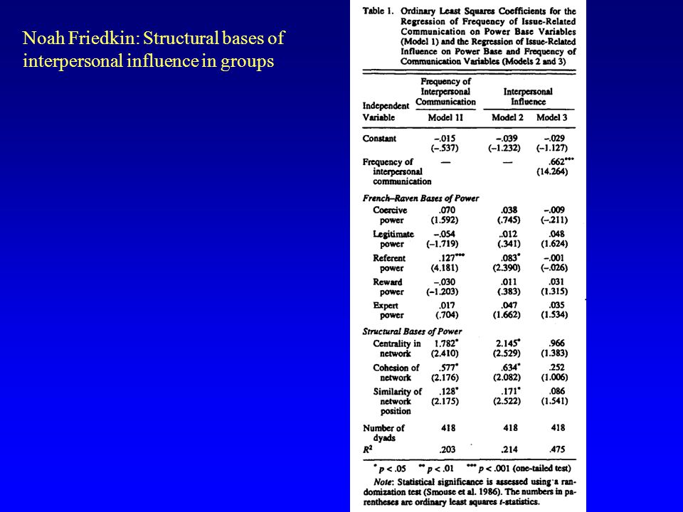
43
Noah Friedkin: Structural bases of interpersonal influence in groups Interested in identifying the structural bases of power. In addition to resources, he identifies: Cohesion Similarity Centrality Which are thought to affect interpersonal visibility and salience

44
Cohesion Members of a cohesive group are likely to be aware of each others opinions, because information diffuses quickly within the group. Groups encourage (through balance) reciprocity and compromise. This likely increases the salience of opinions of other group members, over non-group members. Actors P and O are structurally cohesive if they are joint members of a cohesive group. The greater their cohesion, the more likely they are to influence each other. Note some of the other characteristics he identifies (p.862): Inclination to remain in the group Members capacity for social control and collective action Are these useful indicators of cohesion? Noah Friedkin: Structural bases of interpersonal influence in groups
 reciprocity and compromise. This likely increases the salience of opinions of other group members, over non-group members. Actors P and O are structurally cohesive if they are joint members of a cohesive group. The greater their cohesion, the more likely they are to influence each other. Note some of the other characteristics he identifies (p.862): Inclination to remain in the group Members capacity for social control and collective action Are these useful indicators of cohesion. Noah Friedkin: Structural bases of interpersonal influence in groups.")
45
Structural Similarity Two people may not be directly connected, but occupy a similar position in the structure. As such, they have similar interests in outcomes that relate to positions in the structure. Similarity must be conditioned on visibility. P must know that O is in the same position, which means that the effect of similarity might be conditional on communication frequency.

46
Noah Friedkin: Structural bases of interpersonal influence in groups Centrality Central actors are likely more influential. They have greater access to information and can communicate their opinions to others more efficiently. Research shows they are also more likely to use the communication channels than are periphery actors.

47
Noah Friedkin: Structural bases of interpersonal influence in groups French & Raven propose alternative bases for dyadic power: 1.Reward power, based on P’s perception that O has the ability to mediate rewards 2.Coercive power – P’s perception that O can punish 3.Legitimate power – based on O’s legitimate right to power 4.Referent power – based on P’s identification w. O 5.Expert power – based on O’s special knowledge Friedkin created a matrix of power attribution, b k, where the ij entry = 1 if person i says that person j has this base of power.

48
Noah Friedkin: Structural bases of interpersonal influence in groups Substantive questions: Influence in establishing school performance criteria. Data on 23 teachers collected in 2 waves Dyads are the unit of analysis (P--> O): want to measure the extent of influence of one actor on another. Each teacher identified how much an influence others were on their opinion about school performance criteria. Cohesion = probability of a flow of events (communication) between them, within 3 steps. Similarity = pairwise measure of equivalence (profile correlations) Centrality = TEC (power centrality)
: want to measure the extent of influence of one actor on another. Each teacher identified how much an influence others were on their opinion about school performance criteria. Cohesion = probability of a flow of events (communication) between them, within 3 steps. Similarity = pairwise measure of equivalence (profile correlations) Centrality = TEC (power centrality).")
49
Total Effects Centrality (Friedkin). Very similar to the Bonacich measure, it is based on an assumed peer influence model. The formula is: Where W is a row-normalized adjacency matrix, and is a weight for the amount of interpersonal influence

50
Find that each matter for interpersonal communication, and that communication is what matters most for interpersonal influence. + + + Noah Friedkin: Structural bases of interpersonal influence in groups

52
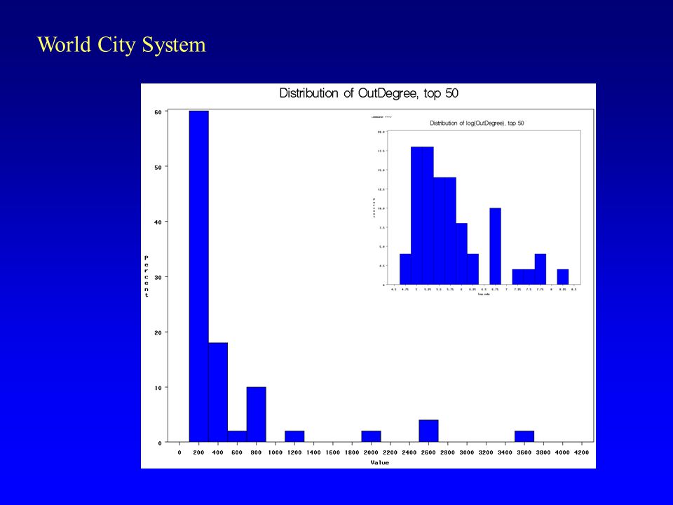
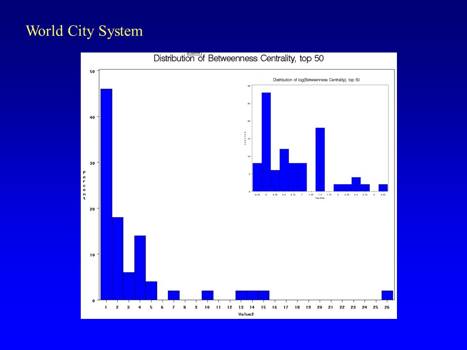
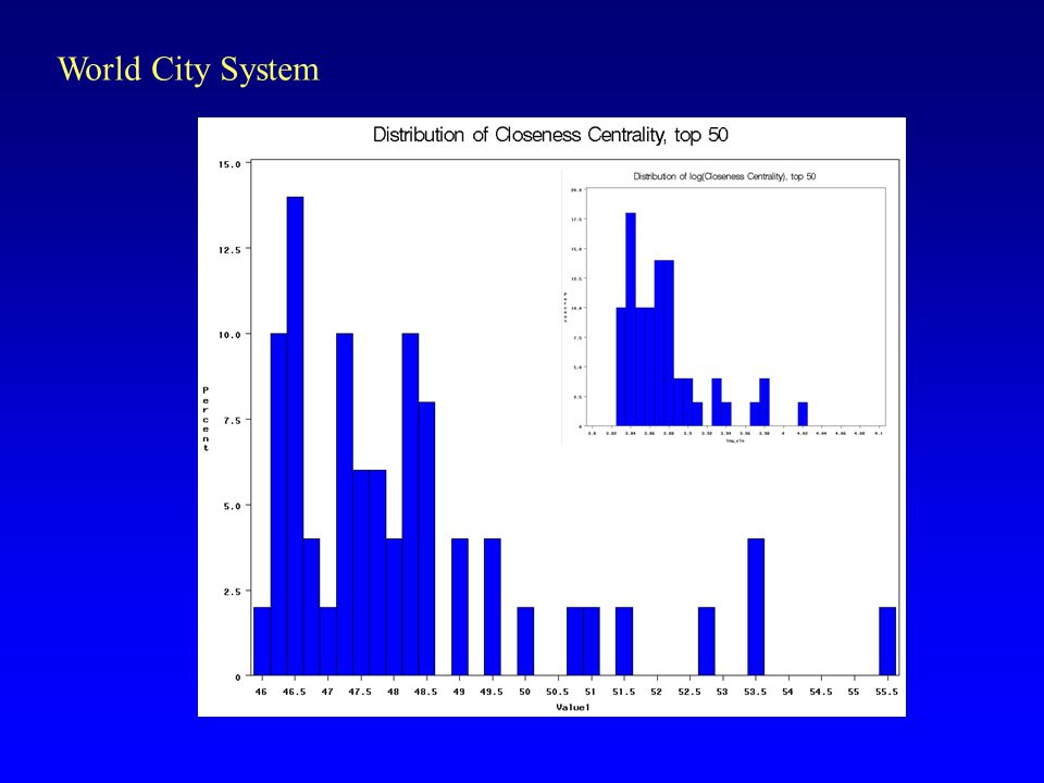
World City System

56
Relation among centrality measures (from table 3) Ln(out-degree) Ln(Betweenness) Ln(Closeness) Ln(In-Degree) r=0.88 N=41 r=0.88 N=33 r=0.62 N=26 r=0.84 N=32 r=0.62 N=25 r=0.78 N=40
 Ln(out-degree) Ln(Betweenness) Ln(Closeness) Ln(In-Degree) r=0.88 N=41 r=0.88 N=33 r=0.62 N=26 r=0.84 N=32 r=0.62 N=25 r=0.78 N=40")
57
World City System

58
Centrality & Aggression Faris & Felmlee, ASR

59
Centrality & Aggression Faris & Felmlee, ASR

60
Multiple cross- gender friends

Similar presentations

 in a network, usually denoted as k or n Size is critical for the structure.>")


