1. Forecasting Financial Time Series using Neural Networks, Genetic Programming and AutoRegressive Models

2. Mohammad Ali Farid 2003-02-0111 Faiza Ather 2003-02-0057 M. Omer Sheikh 2003-02-0129 Umair H. Siddiqui 2003-02-0206

3. Financial time series data : non linear non trivial Stochastic data makes prediction difficult Efficient Market Hypothesis AIM of the project : To test the predictability of financial time series data using both parametric and nonparametric models

4. EFFICIENT MARKET HYPOTHESIS The possibility of arbitrage makes it impossible to predict the future values The prediction which is realized by everyone in the market will not turn true Assumes that every investor has perfect and equal information If EMH is true then investing in speculative trade is no better than gambling If EMH is NOT true then the market can be predicted

5. AGENDA Understanding the Data : Data Analysis Modeling and Prediction Using: Neural Networks Econometrical Methods Genetic Programming Conclusion

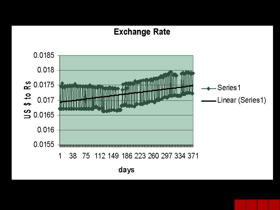
6. DATA SET FINANCIAL TIME SERIES: Daily Exchange Rate DATA: Exchange Rate between US Dollar and Pakistani Rupee. SERIES: 371 Points FROM 31 Jan 2002 to 4 th Feb 2003 ( Period Selected due to stability and lack of external shocks) DATA PROVIDERS: ONADA Currency Exchange

8. DATA ANALYSIS PROBLEM: Non Stationarity 2% difference in mean between the first half and second half SOLUTION: Preprocessing Mean0.01792 Min0.01795 Max0.0013 Range0.001

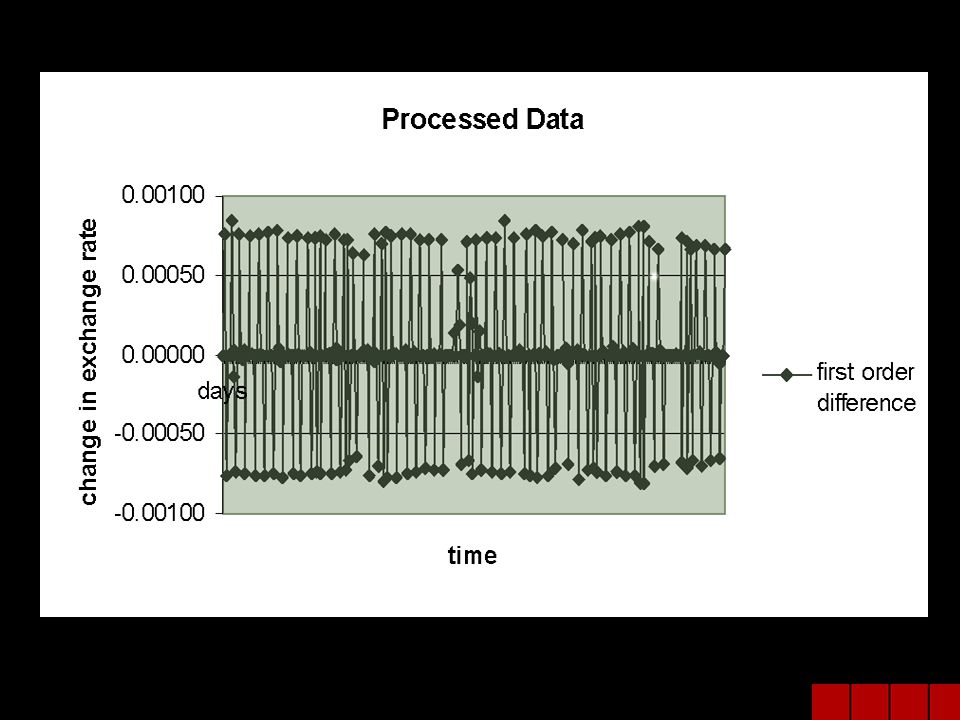
9. DATA PREPROCESSING Unprepocessed data exhibits non - stationarity The trend does not allow modeling First Order Differencing required

11. STATISTICAL ANALYSIS Mean : 3.21622E-06 Standard deviation: 0.000414274 Skewness: -0.008169076 (negatively skewed) Kurtosis: 0.214044239 (leptokurtic) Min: -0.00081 Max: 0.00085 Range: 0.00166

12. MODELING EXCHANGE RATE Numerous factors affect exchange rates Impossible to factor in all the variables Solution: Use Correlation Use past values to predict the future

14. Data Sets Windowing: Selecting the input and output set The project used five different types of data sets for the training. The variations in the data are based on different window sizes and different level of data processing.

15. DATA SETS Data sets used for modeling were: Data Set A: Primary series, change in exchange rate, daily values with 7-1 window. Data Set B: Primary series with 14-1 window. Data Set C: Moving averages, average of three days with 7-1 window. Data Set D: Primary series with 7-3 window.

16. MODELING AND PREDICTION USING NEURAL NETWORKS Feed Forward Networks Radial Basis Networks Recurrent Elman Networks

17. COMPARISON OF DATA SET A AND DATA SET B

18. FEED FORWARD NETWORKS Universal Approximators: Capable of representing non-linear functional mappings between inputs and outputs Can be trained with a powerful and computationally efficient training algorithm called the Error Back Propagation Architecture:

19. COMPARISON OF ALL THE FFNs FFNS with varied: Activation Functions, Training algorithms and number of hidden layers

20. FEED FORWARD NETWORKS BEST: Single hidden layer Activation function: logsig and linear Training algorithm:gradient descent with momentum

21. What are radial basis networks? Radial Basis Function Networks are based on the viewpoint that learning is similar to finding a surface in a multi-dimensional space that provides a best fit to the training data Hidden units provide a set of “functions” that constitute an arbitrary “basis” for the input patterns when they are expanded into the hidden-unit space; these functions are called radial-basis functions. Architecture : The input layer: source nodes. The hidden layer: high enough dimension The output layer: supplies a response of the network to the activation patterns applied to the input layer. RADIAL BASIS NETWORK

22. In the radial basis network the Gaussian function was used as the basis function in its hidden layer Φ (r) = exp ( - r 2 / 2σ 2 ) for σ> 0, & r >= 0 (σ ) Spread of the radial basis is a significant factor in design of the network RADIAL BASIS NETWORK

23. COMPARISON OF RADIAL BASIS NETWORKS RB4 spread = 0.3 RB5 spread = 1.5

24. RADIAL BASIS NETWORK BEST: ( σ ) Spread = 0.3 i.e 1/3 * range

25. RECURRENT ELMAN NETWORKS A modification of the feedforward architecture A “context” layer is added, which retains information between observations. New inputs are fed into the RNN that is, previous contents of the hidden layer are passed into the context layer. These are then fed back into the hidden layer in the next time step

26. COMPARISON OF ELMAN NETWORK

27. RESULTS WITH ELMAN NETWORK BEST: Elman 7 Hidden layers : 2 ; 10 neurons in the first and 5 in the second Activation function for both layers: logsigmoid Training algorithm: gradient descent with momentum

28. A COMPRISON OF ALL THE NEURAL NETS

29. AUTO REGRESSIVE MODEL WITH 16 LAGS

30. CoefficientsStandard Errort StatP-value Intercept 3.3379E-061.49772E-050.2228654670.82380098 deltaE-1 -0.53614060.059802398-8.9652024224.3215E-17 deltaE-2 -0.67117970.06485542-10.348860621.6942E-21 deltaE-3 -0.5559140.072150313-7.7049430182.2207E-13 deltaE-4 -0.54013520.072512856-7.4488197711.1451E-12 deltaE-5 -0.48304570.072841586-6.6314554871.6817E-10 deltaE-6 -0.38021480.067213929-5.6567850843.7728E-08 deltaE-7 0.056051060.0648076730.8648830950.38783548 deltaE-8 0.000331060.0002646661.2508530310.21202124 deltaE-9 0.179177030.0646860182.7699499350.00597734 deltaE-10 0.036592150.071904990.5088958560.61122174 deltaE-11 0.005864290.0796569010.0736193730.94136526 deltaE-12 0.052115150.0808746120.6443944130.51984166 deltaE-13 -0.01595580.080653994-0.1978308510.84331943 deltaE-14 0.271225120.0755747283.5888335420.00039134 deltaE-15 0.024519540.0681474480.3598012390.71926413 deltaE-16 0.057861050.0593314740.9752167320.33028562

31. CoefficientsStandard Errort StatP-value Intercept 3.9728E-061.49617E-050.2655293910.79079431 deltaE-1 -0.53650270.059796091-8.9722039044.0525E-17 deltaE-2 -0.65814030.063456716-10.371484391.3937E-21 deltaE-3 -0.55803890.07211119-7.7385899281.7697E-13 deltaE-4 -0.53822590.072480173-7.4258359741.3142E-12 deltaE-5 -0.48285580.072835047-6.6294426271.6929E-10 deltaE-6 -0.37903850.067197314-5.6406795174.0922E-08 deltaE-7 0.066319620.0639410581.0371993020.30052527 deltaE-8 0.000329840.000264641.2463809490.21365165 deltaE-9 0.18247070.0645922212.8249640840.00506371 deltaE-10 0.014634590.0682830340.2143224560.83044941 deltaE-11 -0.02331920.073815763-0.3159112740.75230189 deltaE-12 0.018767030.0732832720.2560888280.79806764 deltaE-13 -0.05005860.072672532-0.6888241760.49149625 deltaE-14 0.233277970.0647820243.6009675480.00037408 deltaE-15 -0.00702090.059978779-0.1170556780.90689867

32. CoefficientsStandard Errort StatP-value Intercept 3.9069E-061.49253E-050.2617671540.79369005 deltaE-1 -0.53772770.058771271-9.1494993941.1306E-17 deltaE-2 -0.65758250.063167939-10.410067571.015E-21 deltaE-3 -0.55770560.071930164-7.7534318321.5927E-13 deltaE-4 -0.53767660.072202835-7.4467513931.1423E-12 deltaE-5 -0.4822980.072553153-6.6475127621.5146E-10 deltaE-6 -0.37955860.066934163-5.6706254913.4884E-08 deltaE-7 0.067350210.0632223341.0652913810.28764576 deltaE-8 0.000328690.0002641.2450537340.21413475 deltaE-9 0.185720210.0582215243.1898892340.00158208 deltaE-10 0.01847690.059772140.3091222420.7574544 deltaE-11 -0.01899780.063809703-0.2977251610.76612985 deltaE-12 0.023024530.0635101250.3625332450.71722228 deltaE-13 -0.04536220.060488544-0.7499297630.45391562 deltaE-14 0.237069160.0560074814.2328123643.1159E-05

33. CoefficientsStandard Errort StatP-value Intercept 5.3747E-061.53562E-050.350003950.72659334 deltaE-1-0.58760060.059256475-9.9162268074.0971E-20 deltaE-2-0.6803070.064774056-10.502769194.8852E-22 deltaE-3-0.5810410.07380917-7.8722056197.2598E-14 deltaE-4-0.53833540.07430736-7.2447116644.0394E-12 deltaE-5-0.4252870.073370157-5.796457081.7877E-08 deltaE-6-0.35786730.068683094-5.2104129043.6124E-07 deltaE-70.157690930.0612455842.5747314280.01053477 deltaE-80.000262890.0002712240.9692683270.33323029 deltaE-90.137559920.0587633762.3409124380.0199237 deltaE-10-0.05927360.058537783-1.0125706210.31212116 deltaE-11-0.11493090.06138785-1.872208980.06219805 deltaE-12-0.09965050.058159115-1.7134115250.08772047 deltaE-13-0.15441770.056322459-2.741672140.00649795

34. CoefficientsStandard Errort StatP-value Intercept 5.1846E-061.55294E-050.3338574110.73873096 deltaE-1 -0.57161360.059634603-9.5852678514.6471E-19 deltaE-2 -0.67807730.065500161-10.352300241.5029E-21 deltaE-3 -0.58834710.074593774-7.8873488916.5106E-14 deltaE-4 -0.58909670.072776238-8.0946299181.6456E-14 deltaE-5 -0.45177960.073552161-6.1423019922.7057E-09 deltaE-6 -0.43152030.063925001-6.7504155878.1548E-11 deltaE-7 0.171654180.0617224992.7810634020.00577668 deltaE-8 0.000159330.0002716130.5866231610.55791795 deltaE-9 0.182500810.0570679543.1979559950.00153887 deltaE-10 -0.01023890.056367934-0.1816438220.85599048 deltaE-11 -0.04451230.056385834-0.7894237210.43051608 deltaE-12 -0.0373350.054138242-0.6896240620.49098784

35. CoefficientsStandard Errort StatP-value Intercept 5.1E-061.55148E-050.3287193840.7426067 deltaE-1 -0.56749150.059280242-9.5730302244.9934E-19 deltaE-2 -0.68040370.065353654-10.411103879.3804E-22 deltaE-3 -0.60112050.072191761-8.3267190013.4016E-15 deltaE-4 -0.59827460.071483851-8.3693675262.5437E-15 deltaE-5 -0.47369010.066275722-7.1472636987.2978E-12 deltaE-6 -0.4325560.063849147-6.7746556997.0203E-11 deltaE-7 0.172161960.061661892.7920318810.00558828 deltaE-8 0.000163850.0002712870.6039882070.54632694 deltaE-9 0.191237910.0555931693.4399533690.00066787 deltaE-10 0.002886430.0530092380.0544514820.95661322 deltaE-11 -0.03165970.053168257-0.5954627060.55200184

36. CoefficientsStandard Errort StatP-value Intercept 5.0708E-061.54973E-050.3272054250.74374939 deltaE-1 -0.56501240.05906779-9.5654908325.1845E-19 deltaE-2 -0.69098990.062818818-10.999728099.6831E-24 deltaE-3 -0.60706570.071418147-8.5001597231.0253E-15 deltaE-4 -0.6171190.06402544-9.638653073.0267E-19 deltaE-5 -0.47478670.066176111-7.1745933796.1208E-12 deltaE-6 -0.43243640.063777495-6.7803920636.7473E-11 deltaE-7 0.177272430.0609934832.9064159980.00393884 deltaE-8 0.000162060.0002709670.5980758680.55025771 deltaE-9 0.201970190.0525317013.8447296760.00014847 deltaE-10 0.011926720.0507319120.2350929730.81430306

37. CoefficientsStandard Errort StatP-value Intercept 5.1056E-061.54714E-050.3300026330.74163623 deltaE-1 -0.56323250.058485059-9.6303652253.1597E-19 deltaE-2 -0.6889660.062124675-11.090054094.6403E-24 deltaE-3 -0.60013150.064936856-9.2417704245.3859E-18 deltaE-4 -0.61631310.063829378-9.655633682.6223E-19 deltaE-5 -0.47437360.066044942-7.1825883795.7861E-12 deltaE-6 -0.43400980.063321982-6.8540146464.3157E-11 deltaE-7 0.175595520.0604762122.9035470050.00397306 deltaE-8 0.000159510.000270310.590118550.5555707 deltaE-9 0.199140590.0510509013.9008242470.00011921

38. AUTO REGRESSIVE MODEL WITH 9 LAGS

39. SkewnessKurtosisK - SL1 Upper Bound0.2436420.6466660.98716695.91871 Lower Bound-0.24553-0.43510.8537281.39064 Original-0.617972.4246230.11410218.09033 SIMULATION TESTS FOR NORMALITY

40. Lag 1Lag 2Lag 3Lag 4 Upper Bound0.1062340.0964680.1021390.091431 Lower Bound-0.09206-0.12212-0.09085-0.10206 Original0.0365450.0113450.0123180.01403 SIMULATION TESTS FOR AUTOCORRELATION

41. Goldfeld Quandt Upper Bound1.433387 Lower Bound0.727431 Original1.093697 SIMULATION TEST FOR HETEROSKEDASTICITY

42. Chow Upper Bound331.4668 Lower Bound309.0579 Original316.7869 SIMULATION TEST FOR STRUCTURAL STABILITY

44. Inspired by Darwin's Theory of Evolution Inventor John Holland: ‘Adaptation in Natural and Artificial Systems’ (1975) Solution: an Evolved Solution Applications: music, military, optimization techniques etc. GENETIC ALGORITHMS

45. Genetic Programming (GP): a branch of GA’s John Koza (1992): GA’s to evolve programs to perform certain tasks LISP programs used Prefix notation GENETIC PROGRAMMING (GP)

46. Generate an initial population of random functions Execute each program Assign a fitness value to the program Create a new population of computer programs by Crossover (sexual reproduction) Mutation Solution is the best computer program in any generation STEPS IN GP

47. TSGP by Mahmoud Kaboudan (School of Business, University of Redlands) Fitness criteria: minimize the sum of squared error (SSE) Variables in the program: data points in Historical (Training) set: T number of data points to Forecast: k data points for ex post Forecast: f population size: p number of generations: g number of explanatory variables: n number of searches desired (to prevent local minima): s GP & FINANCIALTIME SERIES FORECASTING

48. The variables we manipulated Data in Historical set (T) (Increase T  search time increases exponentially) Total points to forecast (k) Population size (p) (interesting observations) Number of generations (g) Upon completion files generated having results of each search A Results files with forecasts based on the best evolved model found RESULTS & OBSERVATIONS

49. RESULTS FROM A SAMPLE RUN T = 80 K = 15 P = 1000 G = 150 N = 7 S = 50

50. T = 80 K = 15 P = 2000 G = 200 N = 14 S = 100 AN IMPORTANT OBSERVATION Reason for the anomaly: Research shows that after some limit it is not useful to use very large populations This is exactly what we have seen from our results

51. CONCLUSION Overview of the Project Neural Networks AutoRegressive Models Genetic Programming Results: Prediction with Radial Basis and Feedforward can give profitable returns Milestones Significance Further research

52. COMPARISON OF ALL MODELS

53. MILESTONES More than 100 neural networks trained and tested First documented study on Pakistani currency market One of the most broad studies on the subject Results can be used for policy making, investment decisions and financial speculative trading Developed a system that can make PROFITS

54. Developing hybrid models to improve the predictability of the system Developing trading rules for investing in the currency market Making the system resilient to external non market shocks FURTHER RESERACH

55. Q & A