1. Dynamics of Giant Kelp Forests: The Engineer of California’s Nearshore Ecosystems Dave Siegel, Kyle Cavanaugh, Brian Kinlan, Dan Reed, Phaedon Kyriakidis, Stephane Maritorena, Steve Gaines, Kristin Landgren UC Santa Barbara Dick Zimmerman & Victoria Hill Old Dominion University

2. Macrocystis pyrifera – Giant Kelp High economic & ecological importance “Ecosystem engineer” of the nearshore ecosystems Source of natural products Dominant canopy forming macroalga in So Cal Highly dynamic Plant lifespans ~ 2.5 years Frond life spans ~ 4 months Fronds growth can be 0.5 m/day

3. Macrocystis & Fish Stocks Growth and mortality regulated by water temp, nutrients, light, depth, bottom type, predation, wave action Kelp biomass data from Kelco visual estimates; Fish observations from Brooks et al 2002 Reed et al. [2006] El Nino PDO Shift

4. Macrocystis Dynamics Growth –Nutrients & seawater temperature Mortality / Disturbance –Wave action (esp. storms), senescence, predation, DOC release, etc. Colonization –Spore dispersal, benthic light levels, depth, substrate type, etc.

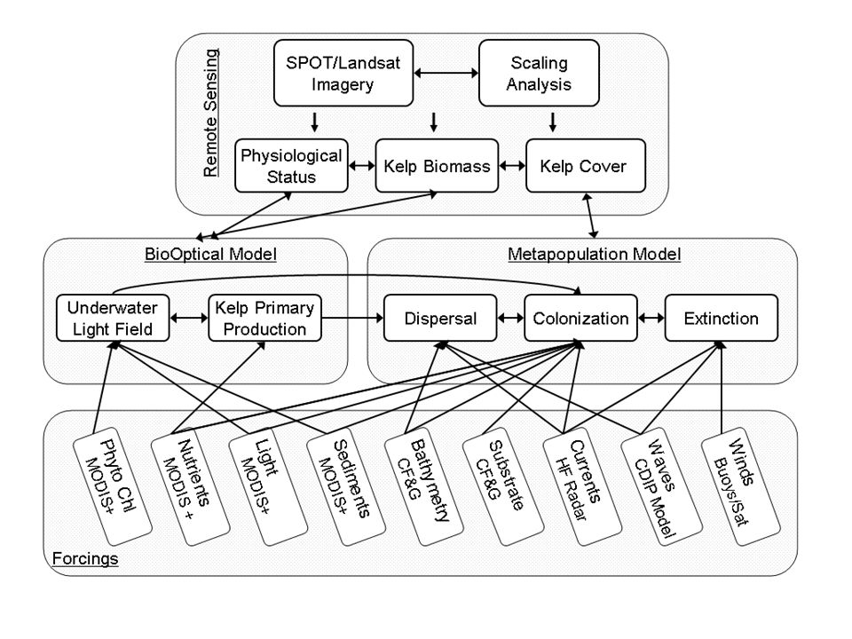
6. Research Goals Understand variability of giant kelp canopy cover & carbon biomass High resolution satellite imagery (SPOT, AVIRIS, etc.) informed by SBC-LTER observations Develop models of kelp forest dynamics Light utilization & gross / net primary production Patch dynamics models of canopy cover

7. Research Area

8. Remote Sensing of Macrocystis with Multispectral Imagery Surface canopy of giant kelp exhibits high near infrared (NIR) reflectance SPOT imagery well suited to differentiate kelp

9. Methods: Canopy Cover 1.Perform dark pixel atmospheric correction 2.Principal components analysis to separate residual surface signal (PC1) from kelp (PC2) PC band 1 PC band 2 False color SPOT image (8/15/2006) Positive contribution from all 3 bands Glint, sediment loads, atmosphere variations, etc. High NIR, low green and red reflectance Kelp

10. Methods: Canopy Cover Classification Minimum kelp threshold value selected from 99.9 th %-tile value of offshore (35-60 m) pixels

11. Validation: Canopy Cover Cover measurements compared with high resolution 2004 CDFG aerial kelp survey SPOT: Oct 29, 2004 CDFG: Sept-Nov 2004 r 2 = 0.98 p ~ 0

12. Kelp Occupation Frequency Jan 2006- May 2007 8 image dates 39% of occupied pixels were present in at least half the scenes ~4% of pixels were present across all dates

13. Kelp Forest Biomass Useful for understanding & modeling ecosystem interactions –NPP, turnover, export, etc. Difficult to measure directly –Time and effort intensive –BUT SBC-LTER does monthly surveys…

14. Research Area

15. SBC-LTER Diver Surveys Monthly measurements of kelp forest attributes at Arroyo Quemado, Arroyo Burro & Mohawk Area Assessment of areal kelp biomass, frond/blade density, net primary production, etc. Sampling for 160 m 2 transect –About 16 SPOT 5 pixels

16. Seasonal kelp biomass changes along 3 LTER transects Maximums in late 2002 Wave driven seasonality apparent

17. Methods: Biomass Normalized Difference Vegetation Index (NDVI) (NIR-RED) (NIR+RED) Calculated for areas of kelp cover NDVI Transform

18. Empirical Estimation of Kelp Biomass from SPOT r 2 = 0.71 Provides path to the remote estimation of kelp biomass (kg/m 2 ) Enables … regional assessment high temporal resolution views with multiple scenes r 2 = 0.71 n = 37

19. Seasonal Kelp Forest Changes

20. Regional Kelp Biomass Created from biomass-NDVI relationship for areas of kelp cover Nov. 2004: 15000 ton Nov. 2006: 7800 ton April 2007: 22350 ton

21. Validation using Visual Biomass Observations r 2 = 0.73 p < 1*10 -7

22. Spectra obtained from airborne inaging spectrometers are similar to lab measures of individual kelp blade reflectances: Optical estimates of kelp physiological state

23. Area and Productivity Estimates Depend on Spatial Resolution Bias increases as spatial resolution decreases Not a linear function of spatial resolution Resolution “classes” result from –inherent scale of kelp patches –spectral averaging as pixel size increases Bias increases as spatial resolution decreases Not a linear function of spatial resolution Resolution “classes” result from –inherent scale of kelp patches –spectral averaging as pixel size increases

24. Metapopulation Modeling >500 m Bed 28 Bed 27 Patch 17 Patch 18 Patch 16 Patch 19

25. Next Steps Acquire as much imagery as possible Characterize kelp forest variability –Patch-level description of occupancy, etc. –Estimate regional scale kelp forest NPP –Assess disturbance factors (waves, etc.) Space/time modeling of kelp cover & biomass –Predict probability of where / when kelp changes –Driven by substrate / disturbance / etc. Compare kelp gross photosynthesis to NPP

26. Thank You!!

27. – 1000 – 100 – 10 – 0 Canopy Biomass (tons/km coast) 36.5°N 35.9°N 35.3°N 34.7°N 34.4°N 34.1°N 33.7°N 33.4°N 32.6°N 32.0°N 31.5°N 30.9°N 30.5°N 29.6°N Lat Location Carmel Bay Pt.Buchon Pt.Purisima Coal Oil Pt. Palos Verdes San Onofre Pt.Loma Pta.San Jose Pta.San Carlos ISP Alginates Visual Kelp Biomass Raw data provided by D. Glantz, ISP Alginates, Inc. & Santa Barbara Coastal LTER Kelp canopy biomass, 34-year monthly time series

28. Regional Kelp Biomass UCSB 11/2004: 15000 metric tons 11/2006: 7800 metric tons 04/2007: 22358 metric tons