1. Bivariate linear regression ASW, Chapter 12 Economics 224 – Notes for November 12, 2008

2. Regression line For a bivariate or simple regression with an independent variable x and a dependent variable y, the regression equation is y = β 0 + β 1 x + ε. The values of the error term, ε, average to 0 so E(ε) = 0 and E(y) = β 0 + β 1 x. Using observed or sample data for values of x and y, estimates of the parameters β 0 and β 1 are obtained and the estimated regression line is where is the value of y that is predicted from the estimated regression line.

3. Bivariate regression line x y E(y) = β 0 + β 1 x yiyi ε or error term xixi y = β 0 + β 1 x + ε E(y i )

4. Observed scatter diagram and estimated least squares line x y ŷ = b 0 + b 1 x y (actual) ŷ (estimated) deviation

5. Example from SLID 2005 According to human capital theory, increased education is associated with greater earnings. Random sample of 22 Saskatchewan males aged 35-39 with positive wages and salaries in 2004, from the Survey of Labour and Income Dynamics, 2005. Let x be total number of years of school completed (YRSCHL18) and y be wages and salaries in dollars (WGSAL42). Source: Statistics Canada, Survey of Labour and Income Dynamics, 2005 [Canada]: External Cross-sectional Economic Person File [machine readable data file]. From IDLS through UR Data Library.

6. ID#YRSCHL18WGSAL42 11762500 21215500 31267500 4119500 51538000 61536000 71970000 81547000 92080000 101628000 111865000 121148000 131472500 141233000 1514.56000 1613.562500 171577500 181342000 191036000 2012.521000 211541000 2212.352500 YRSCHL18 is the variable “number of years of schooling” WGSAL42 is the variable “wages and salaries in dollars, 2004”

7. x y x y Mean of x is 14.2 and sd is 2.64 years. Mean of y is $45,954 and sd is $21,960. n = 22 cases

8. y x

9. Analysis and results H 0 : β 1 = 0. Schooling has no effect on earnings. H 1 : β 1 > 0. Schooling has a positive effect on earnings. From the least squares estimates, using the data for the 22 cases, the regression equation and associate statistics are: y = -13,493 + 4,181 x. R 2 = 0.253, r = 0. 503. Standard error of the slope b 0 is 1,606. t = 2.603 (20 df), significance = 0.017. At α = 0.05, reject H 0, accept H 1 and conclude that schooling has a positive effect on earnings. Each extra year of schooling adds $4,181 to annual wages and salaries for those in this sample. Expected wages and salaries for those with 20 years of schooling is -13,493 + (4,181 x 20) = $70,127.

10. Equation of a line y = β 0 + β 1 x. x is the independent variable (on horizontal) and y is the dependent variable (on vertical). β 0 and β 1 are the two parameters that determine the equation of the line. β 0 is the y intercept – determines the height of the line. β 1 is the slope of the line. –Positive, negative, or zero. –Size of β 1 provides an estimate of the manner that x is related to y.

11. Positive Slope: β 1 > 0 x y β0β0 ΔxΔx ΔyΔy Example – schooling (x) and earnings (y).

12. Negative Slope: β 1 < 0 x y β0β0 ΔxΔx ΔyΔy Example – higher income (x) associated with fewer trips by bus (y).

13. Zero Slope: β 1 = 0 x y β0β0 ΔxΔx Example – amount of rainfall (x) and student grades (y)

14. Infinite Slope: β 1 =  x y

15. Infinite number of possible lines can be drawn. Find the straight line that best fits the points in the scatter diagram.

16. Least squares method (ASW, 469) Find estimates of β 0 and β 1 that produce a line that fits the points the best. The most commonly used criterion is least squares. The least squares line is the unique line for which the sum of the squares of the deviations of the y values from the line is as small as possible. Minimize the sum of the squares of the errors ε. Or, equivalent to this, minimize the sum of the squares of the differences of the y values from the values of E(y). That is, find b 0 and b 1 that minimize:

17. Least squares line Let the n observed values of x and y be termed x i and y i, where i = 1, 2, 3,..., n. ∑ε 2 is minimized when b 0 and b 1 take on the following values:

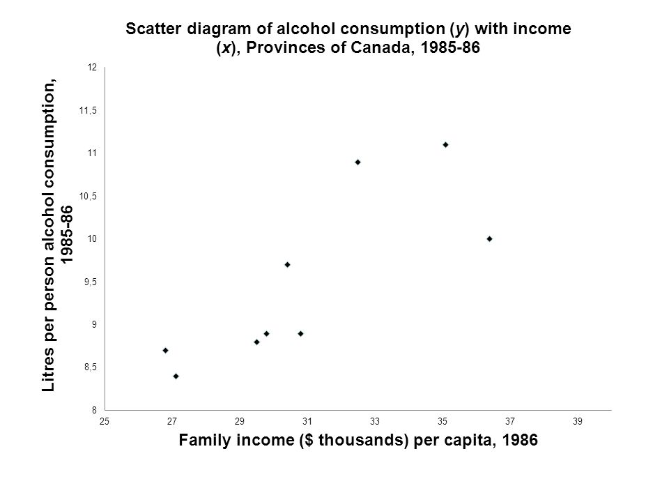
18. ProvinceIncomeAlcohol Newfoundland26.88.7 Prince Edward Island27.18.4 Nova Scotia29.58.8 New Brunswick28.47.6 Quebec30.88.9 Ontario36.410 Manitoba30.49.7 Saskatchewan29.88.9 Alberta35.111.1 British Columbia32.510.9 Income is family income in thousands of dollars per capita, 1986. (independent variable) Alcohol is litres of alcohol consumed per person 15 years of age or over, 1985-86. (dependent variable) Is alcohol a superior good? Sources: Saskatchewan Alcohol and Drug Abuse Commission, Fast Factsheet, Regina, 1988 Statistics Canada, EconomIc Families – 1986 [machine-readable data file, 1988.

19. Hypotheses H 0 : β 1 = 0. Income has no effect on alcohol consumption. H 1 : β 1 > 0. Income has a positive effect on alcohol consumption.

21. Provincexyx-barxy-bary(x-barx)(y-bary)x-barx sq Newfoundland26.88.7-3.88-0.62.32815.0544 PEI27.18.4-3.58-0.93.22212.8164 Nova Scotia29.58.8-1.18-0.50.591.3924 New Brunswick28.47.6-2.28-1.73.8765.1984 Quebec30.88.90.12-0.4-0.0480.0144 Ontario36.4105.720.74.00432.7184 Manitoba30.49.7-0.280.4-0.1120.0784 Saskatchewan29.88.9-0.88-0.40.3520.7744 Alberta35.111.14.421.87.95619.5364 British Columbia32.510.91.821.62.9123.3124 sum306.893-6.8E-14-7.1E-1525.0890.896 mean30.689.3 b10.275919732 b00.834782609

23. SUMMARY OUTPUT Regression Statistics Multiple R0.790288 R Square0.624555 Adjusted R Square0.577624 Standard Error0.721104 Observations10 ANOVA dfSSMSF Significance F Regression16.920067 13.308030.006513 Residual84.1599330.519992 Total911.08 Coefficients Standard Errort StatP-value Intercept0.8347832.3316750.3580180.729592 X Variable 10.275920.0756363.6480180.006513 Analysis. b 1 = 0.276 and its standard error is 0.076, for a t value of 3.648. At α = 0.01, the null hypothesis can be rejected (ie. with H 0, the probability of a t this large or larger is 0.0065) and the alternative hypothesis accepted. At 0.01 significance, there is evidence that alcohol is a superior good, ie. that income has a positive effect on alcohol consumption.

24. Uses of regression line Draw line – select two x values (eg. 26 and 36) and compute the predicted y values (8.1 and 10.8, respectively). Plot these points and draw line. Interpolation. If a city had a mean income of $32,000, the expected level of alcohol consumption would be 9.7 litres per capita.

25. Extrapolation Suppose a city had a mean income of $50,000 in 1986. From the equation, expected alcohol consumption would be 14.6 litres per capita. Cautions: –Model was tested over the range of income values from 26 to 36 thousand dollars. While it appears to be close to a straight line over this range, there is no assurance that a linear relation exists outside this range. –Model does not fit all points – only 62% of the variation in alcohol consumption is explained by this linear model. –Confidence intervals for prediction become larger the further the independent variable x is from its mean.

26. Change in y resulting from change in x Estimate of change in y resulting from a change in x is b 1. For the alcohol consumption example, b 1 = 0.276. A 10.0 thousand dollar increase in income is associated with a 2.76 per litre increase in annual alcohol consumption per capita, at least over the range estimated. This can be used to calculate the income elasticity for alcohol consumption.

27. Goodness of fit (ASW, 12.3) y is the dependent variable, or the variable to be explained. How much of y is explained statistically from the regression model, in this case the line? Total variation in y is termed the total sum of squares, or SST. The common measure of goodness of fit of the line is the coefficient of determination, the proportion of the variation or SST that is “explained” by the line.

28. SST or total variation of y Difference of any observed value of y from the mean is the difference between the observed and predicted value plus the difference of the predicted value from the mean of y. From this, it can be proved that: Difference from mean “Error” of prediction Value of y “explained” by the line SST= Total variation of y SSE = “Unexplained” or “error” variation of y SSR = “Explained” variation of y

29. 29 Variation in y x y ŷ = b 0 + b 1 x yiyi ŷiŷi xixi

30. 30 x y ŷ = b 0 + b 1 x yiyi ŷiŷi xixi Variation in y “explained” by the line “Explained” portion

31. 31 Variation in y that is “unexplained” or error x y yiyi ŷiŷi xixi y i – ŷ i ŷ = b 0 + b 1 x ‘Unexplained” or error

32. Coefficient of determination The coefficient of determination, r 2 or R 2 (the notation used in many texts), is defined as the ratio of the “explained” or regression sum of squares, SSR, to the total variation or sum of squares, SST. The coefficient of determination is the square of the correlation coefficient r. As noted by ASW (483), the correlation coefficient, r, is the square root of the coefficient of determination, but with the same sign (positive or negative) as b 1.

33. Calculations for: ProvincexyPredicted YResidualsSSESSRSST Nfld26.88.78.2294310.4705690.2214351.1461170.36 PEI27.18.48.3122070.0877930.0077080.9757340.81 NS29.58.88.974415-0.174410.030420.1060060.25 NB28.47.68.670903-1.07091.1468330.3957632.89 Que30.88.99.33311-0.433110.1875850.0010960.16 Ont36.41010.87826-0.878260.7713422.4909070.49 Man30.49.79.2227420.4772580.2277750.0059690.16 SK29.88.99.057191-0.157190.0247090.0589560.16 Alb35.111.110.519570.5804350.3369051.4873393.24 BC32.510.99.8021741.0978261.2052220.2521792.56 4.1599336.92006711.08 R squared0.624555

34. SUMMARY OUTPUT Regression Statistics Multiple R0.790288 R Square0.624555 Adjusted R Square0.577624 Standard Error0.721104 Observations10 ANOVA dfSSMSFSignificance F Regression16.920067 13.308030.006513 Residual84.1599330.519992 Total911.08

35. Interpretation of R 2 Proportion, or percentage if multiplied by 100, of the variation in the dependent variable that is statistically explained by the regression line. 0  R 2  1. Large R 2 means the line fits the observed points well and the line explains a lot of the variation in the dependent variable, at least in statistical terms. Small R 2 means the line does not fit the observed points very well and the line does not explain much of the variation in the dependent variable. –Random or error component dominates. –Missing variables. –Relationship between x and y may not be linear.

36. How large is a large R 2 ? Extent of relationship – weak relationship associated with low value and strong relationship associated with large value. Type of data –Micro/survey data associated with small values of R 2. For schooling/earnings example, R 2 = 0.253. Much individual variation. –Grouped data associated with larger values of R 2. In income/alcohol example, R 2 = 0.625. Grouping averages out individual variation. –Time series data often results in very high R 2. In consumption function example (next slide), R 2 = 0.988. Trends often move together.

37. GDP Consumption Consumption (y) and GDP (x), Canada, 1995 to 2004, quarterly data

38. Beware of R 2 Difficult to compare across equations, especially with different types of data and forms of relationships. More variables added to model can increase R 2. Adjusted R 2 can correct for this. ASW, Chapter 13. Grouped or averaged observations can result in larger values of R 2. Need to test for statistical significance. We want good estimates of β 0 and β 1, rather than high R 2. At the same time, for similar types of data and issues, a model with a larger value of R 2 may be preferable to one with a smaller value.

39. Next day Assumptions of regression model. Testing for statistical significance.