1. Randomization/Permutation Tests Body Mass Indices Among NBA & WNBA Players Home Field Advantage in China Soccer League Opponent Effects for 1927 New York Yankees

2. Background Goal: Compare 2 (or More) Treatment Effects or Means based on sample measurements  Independent Samples: Units in different treatment conditions are independent of one another. In controlled experiments they have been randomized to treatments. Observed data are: Y 11,…Y 1n1 and Y 21,…,Y 2n2  Paired Samples: Units are observed under each condition (treatment), and the subsequent difference has been obtained: d j = Y 1j – Y 2j j=1,…,n Procedure: Working under null hypothesis of no differences in treatment effects, how extreme is observed treatment difference relative to many (in theory all) possible randomizations/permutations of the observed data to the treatment labels.

3. Independent Samples – 2 Treatments Algorithm: o Compute Test Statistic for Observed Data and save o Obtain large number of permutations (N) of observed values to treatment labels o For each permutation, compute the Test Statistic and save o P-value = (# Permuted TS ≥ Observed TS)/(N+1)

4. Example – NBA and WNBA Players’ BMI Groups: Male: NBA(i=1) and Female: WNBA(i=2) Samples: Random Samples of n 1 = n 2 = 20 from 2013 seasons (2013/2014 for NBA)

5. Permutation Samples Generate Permutations of the 40 integers using a random number generator (like pulling 1:40 from hat, one-at-a-time without replacement) Assign the first 20 players (based on id) selected to Treatment 1, last 20 to Treatment 2 Compute and save Test Statistic: Continue for many (N total) samples Count number as large or larger than observed Test Statistic (in absolute value, if 2-sided test) P-value obtained as (Count+1)/(N+1)

6. Permutation Samples (EXCEL) Comments:  Column 4: (Ran1) has smallest number (.01077) corresponding to id=11. Thus player 11 is first player in group 1 in Permutation sample. Next smallest is.06690 (id=34)  The “sort” columns (5-8) give the first permutation samples for the 2 groups.  The difference in BMI for groups 1 and 2 in the original sample is 1.5957  The difference in BMI for groups 1 and 2 in the permutation sample is 0.8568

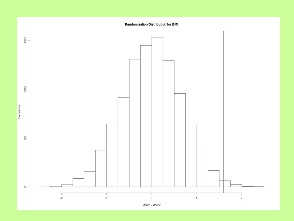
7. R Program ### Download dataset nba.bmi <- read.csv("http://www.stat.ufl.edu/~winner/data/wnba_nba_bmi.csv", header=T) attach(nba.bmi); names(nba.bmi) ### Obtain sample sizes, sample means, and observed Test Statistic (n1 <- length(BMI[Gender==1])); (n2 <- length(BMI[Gender==2])) (ybar1.obs <- mean(BMI[Gender==1])); (ybar2.obs <- mean(BMI[Gender==2])) (TS.obs <- ybar1.obs-ybar2.obs); (n.tot <- n1+n2) ### Choose number of permutations and initialize TS vector to save Test Statistics ### set seed to be able to reproduce permutation samples N <- 9999; TS <- rep(0,N); set.seed(97531) ### Loop through N samples, generating Test Stat each time for (i in 1:N) { perm <- sample(1:n.tot,size=n.tot,replace=F) if (i == 1) print(perm) ybar1 <- mean(BMI[perm[1:n1]]) ### mean BMI of first n1 elements of perm ybar2 <- mean(BMI[perm[(n1+1):(n1+n2)]]) ### mean BMI of next n2 elements of perm TS[i] <- ybar1-ybar2 } ### Count # of cases where abs(TS) >= abs(TS.obs) for 2-sided test and obtain p-value (num.exceed =abs(TS.obs))) (p.val.2sided <- (num.exceed+1)/(N+1)) ### Draw histogram of distribution of TS, with vertical line at TS.obs hist(TS,xlab="Mean1 - Mean2",breaks=seq(-2.5,2.5,0.25), main="Randomization Distribution for BMI") abline(v=TS.obs)

8. R Output > ### Obtain sample sizes, sample means, and observed Test Statistic > (n1 <- length(BMI[Gender==1])) [1] 20 > (n2 <- length(BMI[Gender==2])) [1] 20 > (ybar1.obs <- mean(BMI[Gender==1])) [1] 24.94665 > (ybar2.obs <- mean(BMI[Gender==2])) [1] 23.35099 > (TS.obs <- ybar1.obs-ybar2.obs) [1] 1.595653 > (n.tot <- n1+n2) [1] 40 ### First permutation of 1:40 [1] 26 31 12 20 4 28 23 13 2 19 9 35 34 5 16 14 29 11 32 24 39 10 7 3 36 [26] 30 21 27 1 38 17 22 15 25 8 18 6 40 33 37 > ### Count # of cases where abs(TS) >= abs(TS.obs) for 2-sided test and obtain p-value > (num.exceed =abs(TS.obs))) [1] 121 > (p.val.2sided <- (num.exceed+1)/(N+1)) [1] 0.0122

10. Normal t-test (Equal Variances Assumed)

11. t-test for NBA vs WNBA BMI Note: the Permutation and t-tests give the same P-value to 4 decimal places – ≈Normal Data

12. Paired Samples Data Consists of n Pairs of Observations (Y 1j,Y 2j ) j=1,…,n Data are on same subject (individuals matched on external criteria) under 2 conditions (often Before/After) Construct the differences: d j = Y 1j - Y 2j The true population mean difference is:  d =  1 –  2 Wish to test H 0 :  d = 0 with a 1-sided or 2-sided alternative

13. Procedure Compute an observed Test Statistic that measures the treatment effect in some manner (such as the sample mean of the differences) For many randomization samples:  Generate a series of n U(0,1) random variables: U 1,…,U n  If (say) U j < 0.5 set d j* = -d j where d j* is difference for case j in this sample, otherwise, set d j* = d j  Compute the Test Statistic for this sample and save Compare the observed Test Statistic with the sample Test Statistics in a manner similar to Independent Sample Case: Computing the proportion of sample Test Statistics as extreme or more than the observed Test Statistics

14. Example: English Premier League Football - 2012 Interested in Determining if there is a home field effect  League has 20 teams, all play all 19 opponents Home and Away (190 pairs of teams, each playing once on each team’s home field). No overtime.  Label teams in alphabetical order: 1=Arsenal, 20=Wigan  Let Y 1jk = (H j -A k ) j < k Differential when j at Home, k is Away  Let Y 2jk = (A j -H k ) j < k Differential when j is Away, k is at Home  d jk = Y 1jk – Y 2jk = (H j +H k ) - (A j +A k ) j < k Note: d represents combined Home Goals – Combined Away Goals for the Pair of teams No home effect should mean  d = 0

15. Representative Games from the Sample Comments (regarding these 9 pairs, and these 2 samples - Full Analysis next slide):  For the original sample, the Test Statistic is the Average Difference: 0.556  For the first random sample, games 1,4,8 had Ran1 < 0.5, and their d jk switched sign. The new sampled test statistic was 1.000  For the second random sample, games 1,2,3,5,6,8 had Ran2 < 0.5, and their d jk switched sign. The new sampled test statistic was -0.333  The p-value for a 1-tailed (H A :  d > 0) would be p = (1+1)/(2+1) = 2/3 as both the original sample and Ran1 have Test Statistics ≥ 0.556. The 2-sided is also p = 2/3

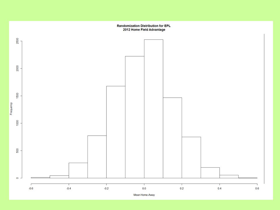
16. R Program epl2012 <- read.csv("http://www.stat.ufl.edu/~winner/data/epl_2012_home_perm.csv", header=T) attach(epl2012); names(epl2012) ### Obtain Sample Size and Test Statistic (Average of d.jk) (n <- length(d.jk)) (TS.obs <- mean(d.jk)) ### Choose the number of samples and initialize TS, and set seed N <- 9999; TS <- rep(0,N); set.seed(86420) ### Loop through samples and compute each TS for (i in 1:N) { ds.jk <- d.jk # Initialize d*.jk = d.jk u <- runif(n)-0.5 # Generate n U(-0.5,0.5)'s u.s 0 ds.jk <- u.s * ds.jk TS[i] <- mean(ds.jk) # Compute Test Statistic for this sample } summary(TS) (num.exceed1 = TS.obs)) # Count for 1-sided (Upper Tail) P-value (num.exceed2 = abs(TS.obs))) # Count for 2-sided P-value (p.val.1sided <- (num.exceed1 + 1)/(N+1)) # 1-sided p-value (p.val.2sided <- (num.exceed2 + 1)/(N+1)) # 2-sided p-value ### Draw histogram of distribution of TS, with vertical line at TS.obs hist(TS,xlab="Mean Home-Away",main="Randomization Distribution for EPL 2012 Home Field Advantage") abline(v=TS.obs)

17. R Output > > ### Obtain Sample Size and Test Statistic (Average of d.jk) > (n <- length(d.jk)) [1] 190 > (TS.obs <- mean(d.jk)) [1] 0.6368421 > > summary(TS) Min. 1st Qu. Median Mean 3rd Qu. Max. -0.573700 -0.110500 -0.005263 -0.002513 0.100000 0.542100 > (num.exceed1 = TS.obs)) # Count for 1-sided (Upper Tail) P-value [1] 0 > (num.exceed2 = abs(TS.obs))) # Count for 2-sided P-value [1] 0 > (p.val.1sided <- (num.exceed1 + 1)/(N+1)) # 1-sided p-value [1] 1e-04 > (p.val.2sided <- (num.exceed2 + 1)/(N+1)) # 2-sided p-value [1] 1e-04 The observed Mean difference (0.6368) exceeded all 9999 sampled values: (min = -0.5737, max = 0.5421) Thus, both P-values = (0+1)/(9999+1) =.0001

19. Normal Paired t-test

20. Paired t-test for EPL 2012 Home vs Away Goals Note: the t-test gives smaller P-value, but Permutation test was limited to number of samples