1. Image Resolution
Chapter 10

2. Definitions Resolution – ability to record and display detail Spatial
Spectral
Radiometric

3. Definitions Spatial resolution – the amount of geometric detail
How close can two points be before you can’t distinguish them

4. Spatial Resolution High spatial resolution: 0.6 - 4 m
» GeoEye-1
» WorldView-2
» WorldView-1
» QuickBird
» IKONOS
» FORMOSAT-2
» ALOS
» CARTOSAT-1
» SPOT-5
Medium spatial resolution: m
» ASTER
» LANDSAT 7
» CBERS-2
Low spatial resolution: 30 - > 1000 m
SeaWiFS
GOES

6. Radiometric Resolution
Radiometric resolution – the amount of brightness detail
Is the image black and white, shades of grey
How many bits – 4, 8, 12, 16, etc.

7. Radiometric Resolution

8. 6 bit
8 bit

9. 2 bit
1 bit

10. 2-bit
8-bit

11. Spectral Resolution
Spectral resolution – the amount of detail in wavelength
2 bands, 4, 6, 200 or more

13. Temporal Resolution Temporal resolution – the amount of detail in time
High altitude aerial photos every 10 years, Landsat 16 days, NOAA 4 hrs
High resolution: < 24 hours - 3 days
Medium resolution: days
Low resolution: > 16 days

15. Tradeoffs

16. Tradeoffs
There are trade-offs between spatial, spectral, and radiometric resolution
Taken into consideration when engineers design a sensor.
For high spatial resolution, the sensor has to have a small IFOV (Instantaneous Field of View).
However, this reduces the amount of energy that can be detected as the area of the ground resolution cell within the IFOV becomes smaller.
This leads to reduced radiometric resolution - the ability to detect fine energy differences.

17. Tradeoffs
To increase the amount of energy detected (and the radiometric resolution) without reducing spatial resolution, we have to broaden the wavelength range detected for a particular channel or band.
Unfortunately, this reduces the spectral resolution of the sensor.
Conversely, coarser spatial resolution would allow improved radiometric and/or spectral resolution.
Thus, these three types of resolution must be balanced against the desired capabilities and objectives of the sensor.

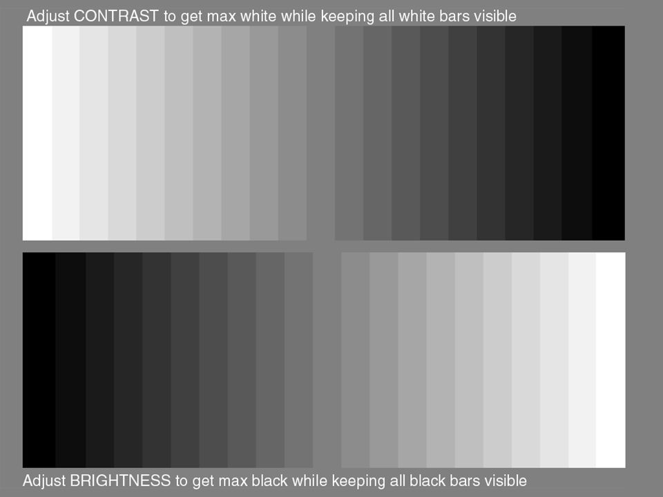
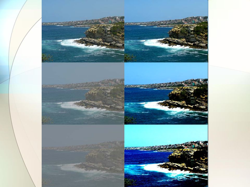
18. Target Variables
Contrast – the brightness difference between an object and the background
High contrast improves spatial detail

21. Contrast versus spatial frequency
Sinusoidal target with varying contrast in % and varying spatial frequency left to right
Obvious resolution decrease from left to right. If your eyes are too good squint to see effect
Picture from

22. Target Variables Shape is also a significant factor
Aspect ratio is how long the object is compared to its width
Long thin features can be seen even if they are narrower than the spatial resolution
Regularity of shape makes for better detail
Agricultural fields

23. Target Variables Number of objects favor higher detail
Orchard versus single tree
Extent and uniformity of background also helps distinguish things

24. Aerial view of Olympic Peninsula facing west from Port Orchard Bay

25. System Variables Design of sensor and its operation are important too
Air photo – have to consider quality of camera and lens, choice of film, altitude, scale,

26. Operating conditions
Altitude
Ground speed
Atmospheric conditions

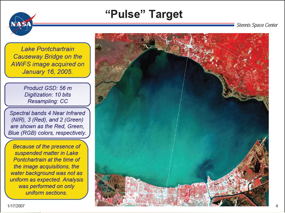
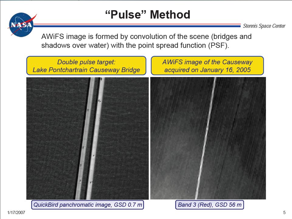
27. Measuring resolution
Ground Resolved Distance (GRD) the dimensions of the smallest objects recorded
Line pairs per millimeter (LPM) is derived from targets
Target is placed on the ground and imaged
If two obejcts are are visually separated, they are considered “spatially resolved”

29. Measuring resolution
Using the target you measure the smallest pair of lines (black line plus adjacent white space)

32. Modulation Transfer Function
The Modulation Transfer Function (MTF) is response of a system to an array of elements with varying spaces

33. Modulation Transfer Function
For low spatial frequencies, the modulation transfer function is close to 1 (or 100%)
generally falls as the spatial frequency increases until it reaches zero.
The contrast values are lower for higher spatial frequencies .
As spatial frequency increases, the MTF curve falls until it reaches zero.
This is the limit of resolution for a given optical system or the so called cut off frequency (see figure below).
When the contrast value reaches zero, the image becomes a uniform shade of grey.

34. Modulation Transfer Function

35. Modulation Transfer Function
The figure represents a sine pattern (pure frequencies) with spatial frequencies from 2 to 200 cycles (line pairs) per mm.
The top half of the sine pattern has uniform contrast.

36. Modulation Transfer Function
Perceived image sharpness (NOT lp/mm resolution) is closely related to the spatial frequency where MTF is 50% (0.5)
i.e. where contrast has dropped by half.

37. Modulation Transfer Function
Contrast levels from 100% to 2% are illustrated on the chart for a variable frequency sine pattern.
Contrast is moderately attenuated for MTF = 50% and severely attenuated for MTF = 10%.
The 2% pattern is visible only because viewing conditions are favorable:
it is surrounded by neutral gray, it is noiseless (grainless), and the display contrast for CRTs and most LCD displays is relatively high.
It could easily become invisible under less favorable conditions.

38. Modulation Transfer Function
How is MTF related to lines per millimeter resolution?
The old resolution measurement— distinguishable lp/mm— corresponds roughly to spatial frequencies where MTF is between 5% and 2% (0.05 to 0.02).
This number varies with the observer, most of whom stretch it as far as they can.
An MTF of 9% is implied in the definition of the Rayleigh diffraction limit.

39. Mixed Pixels
If the area covered by a pixel is not uniform in composition it leads to mixed pixels.
These often occur at the edge of large parcels, along linear features, or scattered due to small features in the landscape (ponds, buildings, vehicles, etc.)

40. Mixed Pixels

42. Mixed Pixels
The spectral responses of those mixed pixels is not a pure signature, but rather, a composite signature
Can you think of an advantage to having a composite signature?
Identify areas that are too complex to resolve individually

43. As resolution becomes coarser
There have been a number of studies on the effect of resolution on mixed pixels
As resolution becomes coarser
Mixed pixels increase
Interior pixels decrease
Background pixels decrease

44. Resolution and Mixed Pixels
Total
Mixed
Interior
Back-ground
A - fine
900 %
109
1.1
143
15.9
648 72 B
225 59
26.2 25
11.1
141
62.7 C
100 34 6 60
D - coarse 49 23
46.9 1 2 51

45. Original Landsat image
Image resampled at coarser resolution
wheat (red), potatoes (green) and sugar beet (blue)

46. Spatial and Radiometric Resolution
Sensors are designed with specific levels of radiometric resolution and spatial resolution
Both of these determine the ability to portray features in the landscape
Broad levels of resolution may be adequate for coarse-textured landscape
Finer resolution may help to identify more features, but may also add more detail than necessary

47. Interactions with Landscape
In a study of field size in grain-producing regions, Podwysocki (1976) showed how effectiveness of different resolutions could be quantified.

48. Interactions with Landscape
Simonett and Coiner (1971) conducted another study to determine the effectiveness of the yet to be launched MSS sensor
Simulated by using airphotos and overlaying a grid of 800, 400, 200, and 100 feet.
Assessed the number of land-use categories in each cell