1. Computer Vision Spring 2006 15-385,-685 Instructor: S. Narasimhan Wean 5403 T-R 3:00pm – 4:20pm Lecture #15

2. Binocular Stereo - Calibration Lecture #15

3. Binocular Stereo

4. Stereo Reconstruction - RECAP The Stereo Problem –Shape from two (or more) images –Biological motivation knowncameraviewpoints

5. Disparity and Depth - RECAP scene left image right image baseline Assume that we know corresponds to From perspective projection (define the coordinate system as shown above)

6. Disparity and Depth - RECAP is the disparity between corresponding left and right image points disparity increases with baseline b inverse proportional to depth scene left image right image baseline

7. field of view of stereo Vergence one pixel uncertainty of scenepoint Optical axes of the two cameras need not be parallel Field of view decreases with increase in baseline and vergence Accuracy increases with baseline and vergence

8. Binocular Stereo Calibration RELATIVE ORIENTATION: We need to know position and orientation of one camera with respect to the other, before computing depth of scene points. ABSOLUTE ORIENTATION: We may need to know position and orientation of a stereo system with respect to some external system (for example, a 3D scanner).

9. Binocular Stereo Calibration - Notation Left Camera Frame Right Camera Frame We need to transform one coordinate frame to another. The transformation includes a rotation and a translation: : Translation of Left frame w.r.t Right : Rotation of Left frame w.r.t Right

10. Binocular Stereo Calibration - Notation In matrix notation, we can write as:

11. Binocular Stereo Calibration - Notation We can expand as:

12. Orthonormality Constraints (a) Rows of R are perpendicular vectors (b) Each row of R is a unit vector NOTE: Constraints are NON-LINEAR! They can only be used once (do not change with scene points).

13. Absolute Orientation We have measured some scene points using Stereo System L and Stereo System R Find Orientation (Translation and Rotation) of system L w.r.t system R. Useful for merging partial depth information from different views. Left System L Right System R Problem: Given Find

14. How many scene points are needed? Each scene point gives 3 equations: Six additional equations from orthonormality of Rotation matrix For n scene points, we have (3n + 6) equations and 12 unknowns It appears that 2 scene points suffice. But orthonormal constraints are non-linear. THREE NON-COLLINEAR SCENE POINTS ARE SUFFICIENT (see Horn)

15. Solving an Over-determined System Generally, more than 3 points are used to find the 12 unknowns Formulate Error for scene point i as: Find that minimize: Orthonormality Constraint

16. Relative Orientation

17. Find Orientation (Translation and Rotation) between two cameras (within the same stereo system). We must do this before using the stereo system. Left Camera L Right Camera R Problem: Here, we DO NOT know both We only know the image coordinates in the two cameras CORRESPOND to the same scene point!

18. Relative Orientation Again, we start with: OR: Assume: we know focal length of both cameras Then: Hence, (same for right camera)

19. Problem Formulation We know: Find: That satisfies : And satisfies the 6 orthonormality constraints

20. Scale Ambiguity Same image coordinates can be generated by doubling Hence, we can find only upto a scale factor! So, fix scale by using constraint: (1 additional equation)

21. How many scene points are needed? If we have n pairs of image coordinates: Number of equations: 3n + 6 + 1 = 3n + 7 Number of unknowns: 2n + 12 n = 5 points will give us equal number of equations & unknowns. In theory, 5 points indeed are good enough if chosen carefully. However, in practice, more points are used and an over-determined system of equations is solved as before.

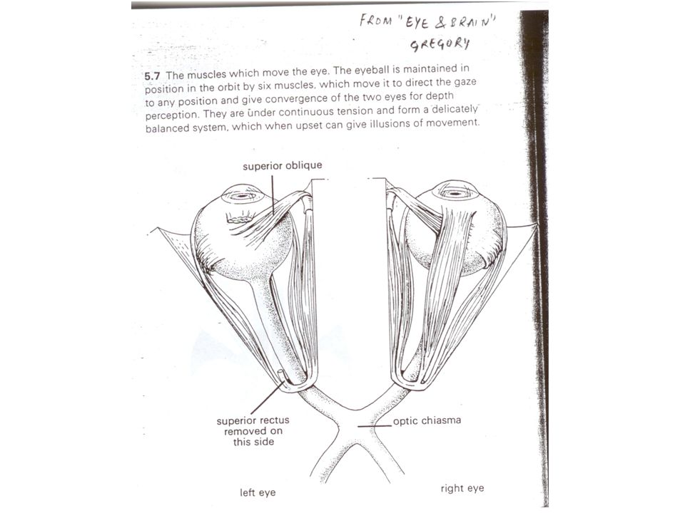
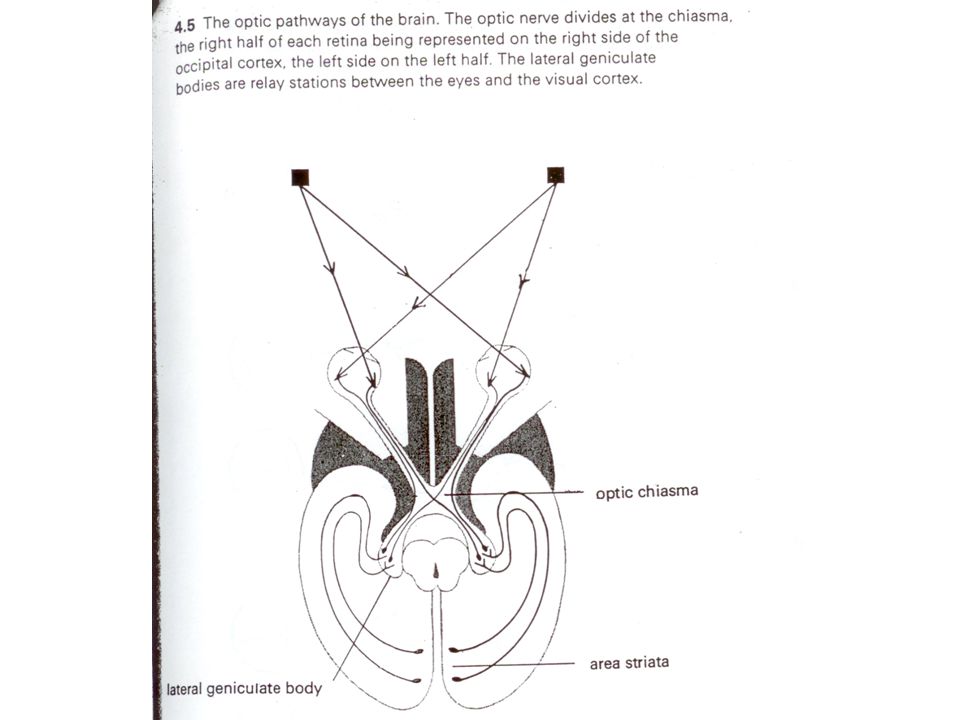
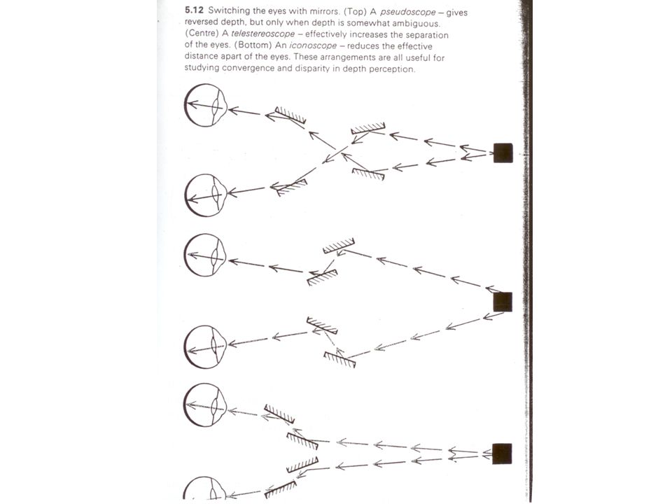
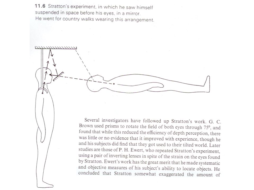
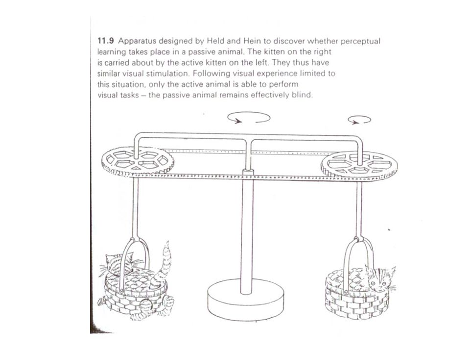
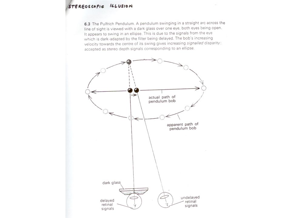
22. Eye and the Brain

30. Next Class Optical Flow and Motion Reading: Horn, Chapter 12.