1. CS 124/LINGUIST 180 From Languages to Information Dan Jurafsky Stanford University Social Networks: Small Worlds, Weak Ties, and Power Laws Slides from Jure Leskovec, Lada Adamic, James Moody, Bing Liu,

2. Networks Information in networks, not just text! Pagerank: the structure of a network tells you something What are the properties of networks and what can we learn from them?

3. Social network analysis Social network analysis is the study of entities (people in an organization), and their interactions and relationships. The interactions and relationships can be represented with a network or graph, each vertex (or node) represents an actor and each link represents a relationship. May be directed or not. CS583, Bing Liu, UIC Nov 5, 2009

4. Various measures of centrality A central actor: involved in many ties. Degree centrality: number of direct connections a node has Prestige centrality: everyone points to this actor: Number of in-links Pagerank is based on prestige Modified from Bing Liu

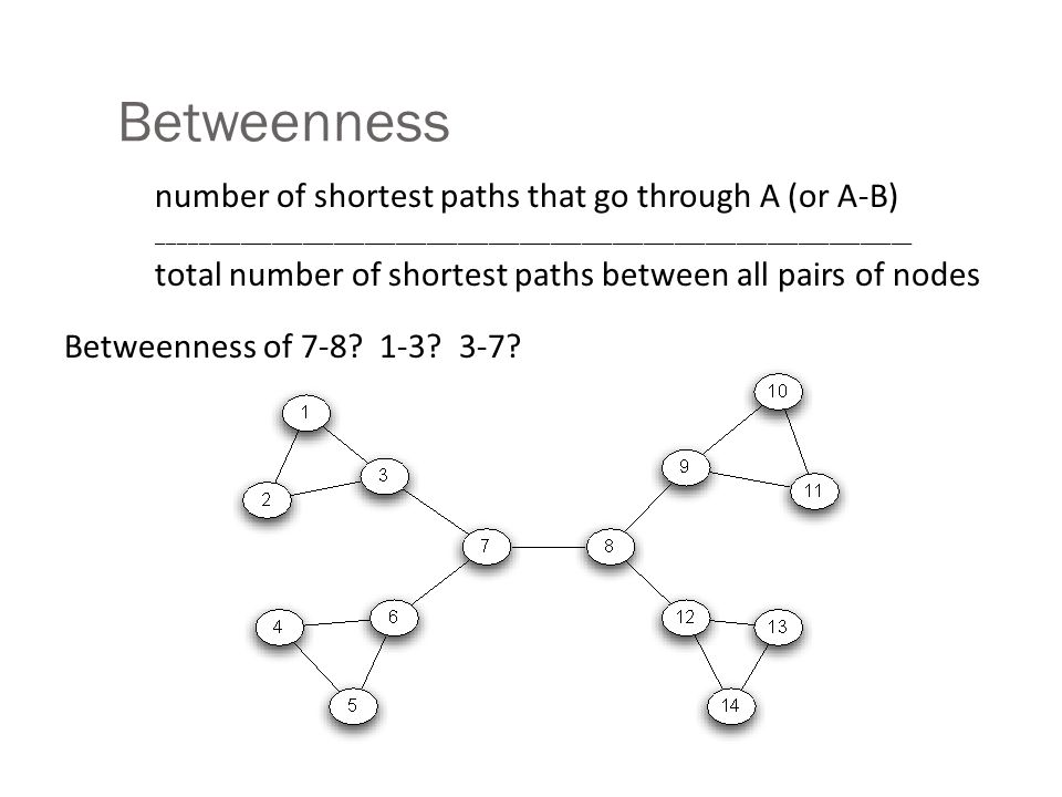
5. Betweenness Centrality The betweenness of a node A (or an edge A-B)= number of shortest paths that go through A (or A-B) ___________________________________________________________________________ total number of shortest paths that exist between all pairs of nodes A node with high betweenness has influence on the network, is a choke-point for information, failure is a problem

6. Betweenness number of shortest paths that go through A (or A-B) _________________________________________________________________________ total number of shortest paths between all pairs of nodes Betweenness of 7-8? 1-3? 3-7?

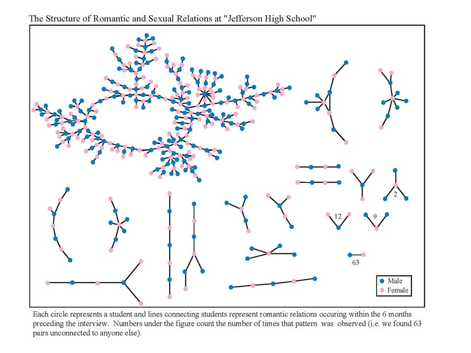
7. An example network Network of which students have had sex with each other in a high school. important for studying disease spread, etc. What do you think its shape is? For example: is it core-periphery (like the web)?

8. High school dating Peter S. Bearman, James Moody and Katherine Stovel Chains of affection: The structure ofChains of affection: The structure of adolescent romantic and sexual networks American Journal of Sociology 110 44-91 (2004) Image drawn by Mark Newman Slide from Drago Radev

10. Why does the graph have this shape? Teens probably don’t say: “By selecting this partner, I maximize the probability of inducing a spanning tree.” The “microtaboo” Bearman and Moody propose don’t date your ex-girlfriend’s boyfriend’s ex-girlfriend (or the reverse) a simulation shows this constraint results in spanning tree

11. CS 124/LINGUIST 180 From Languages to Information Dan Jurafsky Stanford University Small Worlds

12. Small worlds Slide from Lada Adamic

13. Six Degrees of Kevin Bacon Popularization of a small-world idea: The Bacon number: Create a network of Hollywood actors Connect two actors if they co-appeared in the movie Bacon number: number of steps to Kevin Bacon As of 2013, the highest (finite) Bacon number reported is 11 Only approx. 12% of all actors cannot be linked to Bacon Slide adapted from Jure Leskovec

14. Erdös numbers are small too

15. NE MA Chose 300 people in Omaha, NE and Wichita, KA Ask them to get a letter to a stock-broker in Boston by passing it through friends How many steps did it take? The Small World Experiment Slide from Lada Adamic What is the typical shortest path between any two people? Stanley Milgram (1967)

16. Milgram’s small world experiment It took 6.2 steps on average “Six degrees of separation” Can we check this computationally?

17. Facebook 99.6% of all pairs of users connected by paths of 5 degrees (6 hops) 92% are connected by only four degrees (5 hops). Backstrom Boldi Rosa Ugander and Vigna, 2011

18. Duncan Watts: Networks, Dynamics and the Small-World Phenomenon Why do we see the small world pattern? What implications does it has for the dynamical properties of social systems? Slide from James Moody

19. Duncan Watts: Networks, Dynamics and the Small-World Phenomenon Watts says there are 4 conditions that make the small world phenomenon interesting: 1 ) The network is large - O(Billions) 2) The network is sparse - people are connected to a small fraction of the total network 3) The network is decentralized -- no single (or small #) of stars 4) The network is highly clustered -- most friendship circles are overlapping Slide from James Moody

20. Duncan Watts: Networks, Dynamics and the Small-World Phenomenon Formally, we can characterize a graph through 2 statistics. 1)The characteristic path length, L The average length of the shortest paths connecting any two nodes. (Note: this is not quite the same as the diameter of the graph, which is the maximum shortest path connecting any two nodes) 2) The clustering coefficient, C The average local density. A small world graph is any graph with a relatively small L and a relatively large C. Slide from James Moody

21. Local clustering coefficient (Watts&Strogatz 1998) For a vertex i C = The fraction of pairs of neighbors of the node that are connected “What percentage of your friends know each other?” Let n i be the number of neighbors of vertex i number of connections between i’s neighbors maximum number of possible connections between i’s neighbors # directed connections between i’s neighbors n i * (n i -1) # undirected connections between i’s neighbors n i * (n i -1)/2 Slide from Lada Adamic C i = C i directed = C i undirected =

22. Local clustering coefficient (Watts&Strogatz 1998) Average C i over all n vertices Slide from Lada Adamic i n i = 4 max number of connections: 4*3/2 = 6 3 connections present C i = 3/6 = 0.5 link absent link present

23. Watts and Strogatz “Caveman network” Slide from Lada Adamic Everyone in a cave knows each other A few people make connections Are C and L high or low? C high, L high

24. Watts and Strogatz model [WS98] Start with a ring, where every node is connected to the next z nodes ( a regular lattice) With probability p, rewire every edge (or, add a shortcut) to a uniformly chosen destination. Slide from Lada Adamic order randomness p = 0 p = 1 0 < p < 1 Small world

25. Why does this work? Key is fraction of shortcuts in the network In a highly clustered, ordered network, a single random connection will create a shortcut that lowers L dramatically Small world properties can be created by a small number of shortcuts Slide from Lada Adamic

26. Clustering and Path Length Slide from Lada Adamic Regular Graphs have a high clustering coefficient but also a high L Random Graphs have a low clustering coefficient but a low L

27. Small World: Summary Could a network with high clustering be at the same time a small world? Yes! You don’t need more than a few random links The Watts Strogatz Model: Provides insight on the interplay between clustering and the small-world Captures the structure of many realistic networks Accounts for the high clustering of real networks Slide from Jure Leskovec

28. CS 124/LINGUIST 180 From Languages to Information Dan Jurafsky Stanford University Weak links

29. Mark Granovetter (1960s) studied how people find jobs. He found out that most job referrals were through personal contacts But more by acquaintances and not close friends. Aside: Accepted by the American Journal of Sociology after 4 years of unsuccessful attempts elsewhere. One of the most cited papers in sociology. Mystery: Why didn’t jobs come from close friends? Adapted from Drago Radev

30. Triadic Closure “If two people in a social network have a friend in common, then there is an increased likelihood that they will become friends themselves at some point in the future.” (Anatole Rapoport 1953)

31. Reminder: clustering coefficient C C of a node A is the probability that two randomly selected friends of A are friends themselves A before new edge = 1/6 (of B-C, B-D, B-E, C-D, C-E, C-E) After new edge? Triadic closure leads to higher clustering coefficients 2/6

32. Why Triadic Closure? We meet our friends through other friends B and C have opportunity to meet through A B and C’s mutual friendship with A gives them a reason to trust A A has incentive to bring B and C together to avoid stress: if A is friends with two people who don’t like each other it causes stress Bearman and Moody: teenage girls with low clustering coefficients in their network of friends much more likely to consider suicide

33. Bridges A bridge is an edge whose removal places A and B in different components If A is going to get new information (like a job) that she doesn’t already know about, it might come from B

34. Local Bridge A local bridge is an edge whose endpoints A and B have no friends in common (so a local bridge does not form the side of any triangle) If A is going to get new information (like a job) that she doesn’t already know about, it might come from B

35. Strong and Weak Ties Strength of ties amount of time spent together emotional intensity intimacy (mutual confiding) reciprocal services Simplifying assumption: Ties are either strong (s) or weak (w) Adapted from James Moody

36. Strong ties and triadic closure The new B-C edge more likely to form if A-B and A-C are strong ties More extreme: if A has strong ties to B and to C, there must be an edge B-C s s

37. Strong triadic closure If a node Q has two strong ties to nodes Y and Z, there is an edge between Y and Z

38. Closure and bridges If a node A in a network satisfies the Strong Triadic Closure Property and is involved in at least two strong ties, then any local bridge it is involved in must be a weak tie. So local bridges are likely to be weak ties Explaining why jobs came from weak ties

39. Strength of weak ties Weak ties can occur between cohesive groups old college friend former colleague from work Slide from James Moody weak ties will tend to have low transitivity

40. Strength of weak ties – how to get a job Granovetter: How often did you see the contact that helped you find the job prior to the job search 16.7% often (at least once a week) 55.6% occasionally (more than once a year but less than twice a week) 27.8% rarely – once a year or less Weak ties will tend to have different information than we and our close contacts do Long paths rare 39.1 % info came directly from employer 45.3 % one intermediary 3.1 % > 2 (more frequent with younger, inexperienced job seekers) Compatible with Watts/Strogatz small world model: short average shortest paths thanks to ‘shortcuts’ that are non- transitive Slide from James Moody

41. More evidence for strength of weak ties In the Milgram small world experiments, acquaintanceship ties were more effective than family, close friends at passing information

42. Summary Triangles (triadic closure) lead to higher clustering coefficients Your friends will tend to become friends Local bridges will often be weak ties Information comes over weak ties

43. CS 124/LINGUIST 180 From Languages to Information Dan Jurafsky Stanford University Finding paths

44. Watts model shows how these short paths can exist small world networks But how do people find the paths? People seem to be successful by making greedy local decisions The existence of findable short paths depends on further elucidating the structure of the network Slide from Lada Adamic

45. nodes are placed on a lattice and connect to nearest neighbors additional links placed with p uv ~ Spatial search “The geographic movement of the [message] from Nebraska to Massachusetts is striking. There is a progressive closing in on the target area as each new person is added to the chain” S.Milgram ‘The small world problem’, Psychology Today 1,61,1967 Kleinberg, ‘The Small World Phenomenon, An Algorithmic Perspective’ Proc. 32nd ACM Symposium on Theory of Computing, 2000. (Nature 2000) Slide from Lada Adamic

46. Increasing r favors near nodes r=0, Link to each other node equally likely r=1, inverse of distance If a node is twice as far away, 1/2 as likely r=2, inverse squared If a node is twice as far away, 1/4 as likely Slide from Lada Adamic d -r (u,v) =1, Uniform Distribution

47. Kleinberg’s SW network is Greedy Routable iff r=2 Greedy routing algorithm using local information only, find a short path from s to t Slide from Lada Adamic  Starting at the current node u,  choose as next node v the one the closest to t (lattice distance)  whether (u,v) is a local or random edge. s u t v

48. Kleinberg’s SW network is Greedy Routable iff r=2 A greedy routing algorithm using local information only, find a short path from s to t Slide from Lada Adamic u t v s The number of hops is the ‘delivery time’ This greedy routing achieves expected ‘delivery time ’ of O(log 2 n), i.e. the s  t paths have expected length O(log 2 n).

49. Kleinberg’s SW network is Greedy Routable iff r=2 A greedy routing algorithm using local information only, find a short path from s to t Slide from Lada Adamic u t v s This greedy routing achieves expected `delivery time’ of O(log 2 n), i.e. the st paths have expected length O(log 2 n). This does not work unless r=2 : for r2, >0 such that the expected delivery time of any decentralized algorithm is (n  ).

50. Overly localized links on a lattice When r>2 expected search time ~ N (r-2)/(r-1) Slide from Lada Adamic

51. When r=0, links are randomly distributed, ASP ~ log(n), n size of grid When r=0, any decentralized algorithm is at least a 0 n 2/3 no locality When r<2, expected time at least  r n (2-r)/3 Slide from Lada Adamic Good paths exist, but are not greedily findable

52. Links balanced between long and short range When r=2, expected time of a DA is at most C (log N) 2 Slide from Lada Adamic

53. CS 124/LINGUIST 180 From Languages to Information Dan Jurafsky Stanford University Power Laws

54. Degree of nodes Many nodes on the internet have low degree One or two connections A few (hubs) have very high degree The number P(k) of nodes with degree k follows a power law: Where alpha for the internet is about 2.1 I.e., the fraction of web pages with k in-links is proportional to 1/k 2

55. Power-law distributions Right skew normal distribution is centered on mean power-law or Zipf distribution is not High ratio of max to min human heights (max and min not that different) city sizes Power-law distributions have no “scale” (unlike a normal distribution) Slide from Lada Adamic

56. Normal (Gaussian) distribution of human heights Slide from Lada Adamic average value close to most typical distribution close to symmetric around average value

57. Power-law distribution linear scale Slide from Lada Adamic log-log scale high skew (asymmetry) straight line on a log-log plot

58. Power laws are seemingly everywhere note: these are cumulative distributions Slide from Lada Adamic Moby Dick scientific papers 1981-1997AOL users visiting sites ‘97 bestsellers 1895-1965AT&T customers on 1 dayCalifornia 1910-1992

59. Yet more power laws Slide from Lada Adamic MoonSolar flares wars (1816-1980) richest individuals 2003US family names 1990US cities 2003

60. Power law distribution Straight line on a log-log plot Exponentiate both sides to get that p(x), the probability of observing an item of size ‘x’ is given by Slide from Lada Adamic normalization constant (probabilities over all x must sum to 1) power law exponent 

61. What does it mean to be scale free? A power law looks the same no mater what scale we look at it on (2 to 50 or 200 to 5000) Only true of a power-law distribution! p(bx) = g(b) p(x) – shape of the distribution is unchanged except for a multiplicative constant p(bx) = (bx)  = b  x  Slide from Lada Adamic log(x) log(p(x)) x →b*x

62. Many real world networks are power law Slide from Lada Adamic exponent   in/out degree) film actors co-appearance2.3 telephone call graph2.1 email networks1.5/2.0 sexual contacts3.2 WWW2.3/2.7 internet2.5 peer-to-peer2.1 metabolic network2.2 protein interactions2.4

63. Hey, not everything is a power law number of sightings of 591 bird species in the North American Bird survey in 2003. Slide from Lada Adamic cumulative distribution another examples: size of wildfires (in acres)

64. Zipf’s law is a power-law Zipf George Kingsley Zipf how frequent is the 3rd or 8th or 100th most common word? Intuition: small number of very frequent words (“the”, “of”) lots and lots of rare words (“expressive”, “Jurafsky”) Zipf's law: the frequency of the r'th most frequent word is inversely proportional to its rank: y ~ r - , with  close to unity.

65. Pareto’s law and power-laws Pareto The Italian economist Vilfredo Pareto was interested in the distribution of income. Pareto’s law is expressed in terms of the cumulative distribution (the probability that a person earns X or more). P[X > x] ~ x -k Slide from Lada Adamic

66. Income The fraction I of the income going to the richest P of the population is given by Income fraction= (100/P) k-1 if k = 0.5 top 1 percent gets 100 -0.5 =.10 currently k = 0.6 top 1 percent gets 100 -0.4 =.16 (higher k = more inequality)

67. Where do power laws come from? Many different processes can lead to power laws There is no one unique mechanism that explains it all Slide from Lada Adamic

68. Preferential attachment Slide from Lada Adamic Price (1965) Citation networks new citations to a paper are proportional to the number it already has each new paper is generated with m citations new papers cite previous papers with probability proportional to their in-degree (citations)

69. This is a “Rich get Richer” Model Explanation for various power law effects 1. Citations 2. Assume cities are formed at different times, and that, once formed, a city grows in proportion to its current size simply as a result of people having children 3. Words: people are more likely to use a word that is frequent (perhaps it comes to mind more easily or faster)

70. Implications: Wealth Thomas Piketty’s book, #1 on NY Times best seller list last year Focuse on rise of inequality in wealth That same power law An equation from a Stanford economist, wealth is a power low on η:

71. Power laws Many processes are distributed as power laws Word frequencies, citations, web hits Power law distributions have interesting properties scale free, skew, high max/min ratios Various mechanisms explain their prevalence rich-get-richer, etc Explain lots of phenomena we have been dealing with the use of stop words lists (a small fraction of word types cover most tokens in running text)

72. CS 124/LINGUIST 180 From Languages to Information Dan Jurafsky Stanford University Power Laws