1. Diffraction - Deviation of light from rectilinear propagation caused by the obstruction of light waves,.i.e, a physical obstacle. There is no significant physical distinction between interference and diffraction. However, interference generally involves a superposition of only a few waves whereas diffraction involves a large number of waves. Huygens-Fresnel Principle: Every unobstructed point of a wavefront serves as a source of spherical secondary wavelets. The amplitude of the optical field at any point is the superposition of these wavelets. Suppose light strikes a screen containing an aperture. The effects of diffraction can be understood by considering the phasor addition of the electric field for an array of point sources emitting E-M waves that are unobstructed by the aperture. The principles of diffraction can be understood by considering the interference of water waves whose wavelength is made to vary in comparison to the size of the aperture.

2. To illustrate diffraction consider water waves in a ripple tank: Constructive interference of most phasors for all angles; N small  Approx. spherical wave Destructive interference of most phasors for large angles; N large  shadow Intermediate region; N medium, mixed interference N=5 Effective number of point sources N for phasor construction region

3. Light waves striking an aperture Fresnel Diffraction (near-field diffraction) when incoming and outgoing waves are both non- planar. Source S and Screen C are moved to a large distance R, resulting in Fraunhofer diffraction (Far-field diffraction). As a rule-of-thumb: R > a 2 / for Fraunhofer diffraction. Fraunhofer diffraction conditions produced by lenses, leaving source S and screen C in their original position. Note that the lenses act to filter non-plane wave components from striking point P on the observation screen C. Both incoming and outgoing wave contributions are considered as plane waves, and  = const. R a

4. Consider a serious of diffraction measurements on a screen whose distance (R) from the slit varies from close (bottom) to far (top). The diffraction pattern in the near-field (bottom) is sensitive to variations in R whereas the shape is independent of distance for R large (top). The sharp structure shown in the near-field pattern is a result of rapidly changing phasor (E-field) orientations whose summations at each point on the screen are sensitive to distance, slit geometry, and angular spread of the waves. As shown, small changes in R in the near-field can cause large changes in the resulting phasor addition and irradiance distribution on the screen. If a >>, the pattern will resemble a sharp geometric shadow for near-field distances. For large distances (e.g., R 6 > a 2 / ), the parallel nature of the plane waves will result in phasor additions yielding smooth distribution in irradiance, whose shape is independent of R. R1R1 R2R2 R3R3 R4R4 R5R5 R6R6 R 6 > R 5 > R 4 > R 3 …. a

5. As a bridge between interference and diffraction, consider a linear array of equally spaced N coherent point oscillators. We examine the superposition of the fields from each source at a point P sufficiently far such that rays are nearly parallel. The field of each wave is equal so that E 0 (r 1 ) = E 0 (r 2 ) = … = E 0 (r N ) = E 0 (r). In order to evaluate the field, we employ a phasor sum, as follows: Due to a difference in OPL, there is a phase difference between adjacent sources of  = k 0 , where  = ndsin , and  = kdsin . From the figure,  = k(r 2 -r 1 ), 2  = k(r 3 -r 1 ), 3  = k(r 4 -r 1 ), …

6. Therefore, at point P, the phasor sum is obtained using a geometric series (similar to what was done for multiple beam interference) and yields: Note that as   0, I  N 2 I 0, as expected for N coherent sources completely in-phase. Also note that for N = 2, I = 4I 0 cos 2 (  /2) using sin(2  ) = 2sin  cos  and again  = kdsin . This is true for   0 and for  = 2m , m = 0,  1,  2, …

7. For conditions of constructive interference with N sources,  = kdsin  = 2m  (2  / )dsin  m = 2m  which gives dsin  m = m and I m = N 2 I 0, conditions which are identical to two beam interference when there is complete constructive interference. Consider now a line source of oscillators, where each point emits a spherical wavelet as shown in the figure. The electric field for a spherical wavelet emitted from a point is where  0 is the source strength for a point emitter. Let  L = source strength per unit length. Then for each differential segment of source length dy, the contribution of the spherical wavelet at point P is From geometry, from the law of cosines. y (90  -  ) Y Width of line source = D

8. where R >>D and D > y. Note that in order to fulfill Fraunhofer (far-field) diffraction conditions, we also require R > D 2 /. Thus r  R - ysin  is the resulting approximation that we will use. We can calculate the total field appearing on the screen at angle , by summing or integrating all contributions of dE on the linear source: Note that we are also ignoring the presence of ysin  in the denominator since its presence in the phase of the sine in the numerator has a much greater contribution to the integral. We can further separate terms in the sine by using the following identity: Since sin(kysin  ) is an odd function in y, the last term cancels in the integral.

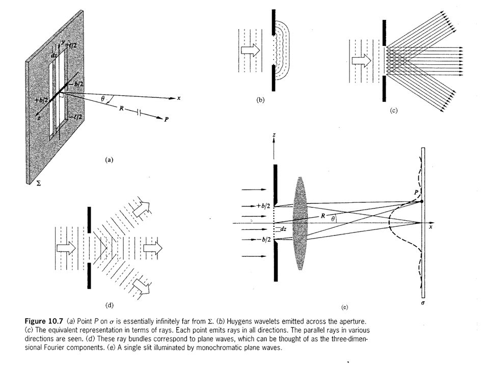
9. Therefore, the integral is as follows: We can now solve the single-slit diffraction problem by considering Figs. 10.6 and 10.7 on the next slides where the variable D  b and  = (kb/2)sin , where b is the slit width (typically a few hundred ) and l is the slit height (typically ~ cm). Clearly, I(  ) have minima when sin  = 0 and  = m , m =  1,  2,  3,… (minima)

10. Note that the condition for diffraction minima, bsin  = m, should not be confused with a similar expression for two-slit interference maxima, asin  = m. Fig. 10.6 (a) Single-slit Fraunhofer diffraction. (b) Diffraction pattern of a single vertical slit under point-source illumination. Fraunhofer diffraction using lenses so that the source and fringe pattern can both be at convenient distances from the aperture.

12. We can determine the conditions for maxima in the diffraction pattern by setting the derivative of the Irradiance to zero: The first condition (i) is just the condition for minima that we have already seen (i.e.  = m , m =  1,  2,  3, …) The second condition (ii) results in a transcendental equation whose graphical solutions can be observed on the left. The solutions can easily be found numerically:    1.43 ,  2.46 ,  3.47  …which approaches (m+1/2)  for large .

13. Principal or Central Maximum Subsidiary Maximum (SM) 1 st SM 2 nd SM 3 rd SM Minima (I = 0)

14. Phasor constructions of the E-field for (a) the central maximum, (b) a direction slightly displaced from the central maximum, (c) the first minimum, and (d) the first maximum beyond the central maximum for single-slit diffraction. The example corresponds to N = 18 phasors. For the figure on the far left, the conditions for minima of m = bsin  are understood by dividing the phasors of rays in two and four equal segments in (b) and (c), respectively. In (b), for each ray in the top half, a phasor 180  out-of-phase can be found in the bottom half, resulting in zero E- field. Likewise, in (c), each successive quarter contains phasors that are 180  out- of-phase, resulting in zero E-field and zero irradiance.

15. Figure 10.13 (a) Double-slit geometry. Point P on the screen  is essentially infinitely far away. (b) A double-slit diffraction pattern for a =3b. Consider now the set-up for a double-slit diffraction measurement. The rectangular geometry of the slit is shown such that l >> b, where l and b are the height and width of each slit. The screen on which the diffraction pattern is observed is located a distance R from the slits, where R >> a and R >> b 2 /. The point P is located on the screen. We will need to calculate the resulting E- field contribution at point P from all points (sources) located in both slits, using essentially the same procedure performed for the single-slit case.

16. The E-field is obtained, as before, by integration over all sources in each slit: Integration procedure is similar to that of the single slit and results in: Note that the definition for  is precisely as before for single-slit diffraction. Using the identity: sin x + sin (x + 2y) = 2cos y sin(x + y), we can express E as After squaring and time-averaging, we obtain the irradiance as: in which  =  = 0 represents  = 0 and I(0) = 4I 0 since E 0 = 2bC and twice that relative to a single slit. Note that I 0 = (bC) 2 = (E 0 /2) 2 is the contribution from one slit.

17. Examine some limits: If kb << 1, (sin  /  )  1 and we get I(  ) = 4I 0 cos 2  = 4I 0 cos 2 (  /2), which yields the expected result for Young’s two slit interference when the slit width b is very small. If a = 0,  = 0, then I(  ) =4I 0 (sin  /  ) 2 = I 0 ’ (sin  /  ) 2, which is just the situation of two slits coalescing into a single slit. Note that the expression I(  ) =4I 0 (sin  /  ) 2 cos 2  is that of an interference term modulated by a diffraction effect. Note that in general for two slits, minima occur when  = m , m =  1,  2,  3, … and  =  (2m+1)  /2, m = 0, 1, 2, 3, … As a general rule-of-thumb, for a = mb, we observe 2m bright fringes within the central diffraction peak, including fractional fringes. So, in Fig. 10.13, for a =3b, we have 5 + 2(1/2) = 6 bright fringes within the central maximum. When an interference maximum overlaps with a diffraction minimum (as shown in Fig. 10.13c) it is often referred to as a missing order.

18. Single- and double-slit Fraunhofer patterns. (a) Photographs taken with monochromatic light. The faint cross-hatching arises entirely in the printing process. (b) When the slit spacing equals b, the two slit coalesce into one (of width 2b) and the single-slit pattern appears (i.e., that’s the first curve closest to you). The farthest curve corresponds to the two slits separated by a =10b. Notice that the two-slit patterns all have their first diffraction minimum at a distance from the central maximum of Z o. Note how the curves gradually match Fig. 10.13(b) as the slit width b gets smaller in comparison to the separation a. (a)(a) (b)(b) Figure 10.14

19. For diffraction from many slits (i.e., the N-slit problem), we generalize the 2-slit problem: The integrals can be evaluated as before for the single- and double-slit cases using the same identities. The result is (see figure for R j )

20. The summation can be evaluated most easily using phasors, as before: Again, the phasor sum is evaluated as a geometric series, as was done for the case of multiple beam interference. Therefore, we can write Therefore, the time-averaged irradiance can be expressed as Note that I 0 is the irradiance in for  = 0 emitted by one slit and I(0) = N 2 I 0, which is seen by taking the limit for  = 0 of the above expression. Also note that if kb << 1 (i.e. very narrow slits), we get the same expression for a linear coherent array of oscillators.

21. The principal maxima are given by the following positions:  = 0, ,  2 ,  3 , … = m  (m = 0,  1,  2,  3..) and  = (ka/2)sin   a sin  m = m and (sinN  /sin  ) 2 = N 2 at these positions. Minima are determined by (sinN  /sin  ) 2 = 0   =  /N,  2  /N,  3  /N, …,  (N-1)  /N,  (N+1)  /N,… Therefore, between consecutive principle maxima we have (N – 1) minima (see figures on next slide). Subsidiary maxima: Between consecutive principle maxima we have (N-2) subsidiary maxima when |sinN  |  1. This occurs for    3  /2N,  5  /2N,  7  /2N, …For large N, sin 2    2 and the intensity of the firs subsidiary peak is approximately Diffraction term multiple-slit interference term

22. Figure 10.17 multiple-slit pattern with a = 4b, N = 6

23. Finally, note that for N = 2 slits, we observe that