1. AOE 5104 Class 2 Online presentations: Homework 1, due in class 9/4
Fundamentals
Algebra and Calculus 1
Homework 1, due in class 9/4
Grading Policy
Study Groups
Recitation times (recitations to start week of 9/8)
Monday 5-6, 5:30-6:30…
Tuesday 5-6, 5:30-6:30…

2. Streamline: Line everywhere tangent to the velocity vector
3a. Ideal Flow
Viscous and compressible effects small (large Re, low M). Flow is a balance between inertia and pressure forces, i.e. acceleration vector balances the pressure gradient vector
Acceleration vector
Pressure gradient vector
Streamline: Line everywhere tangent to the velocity vector

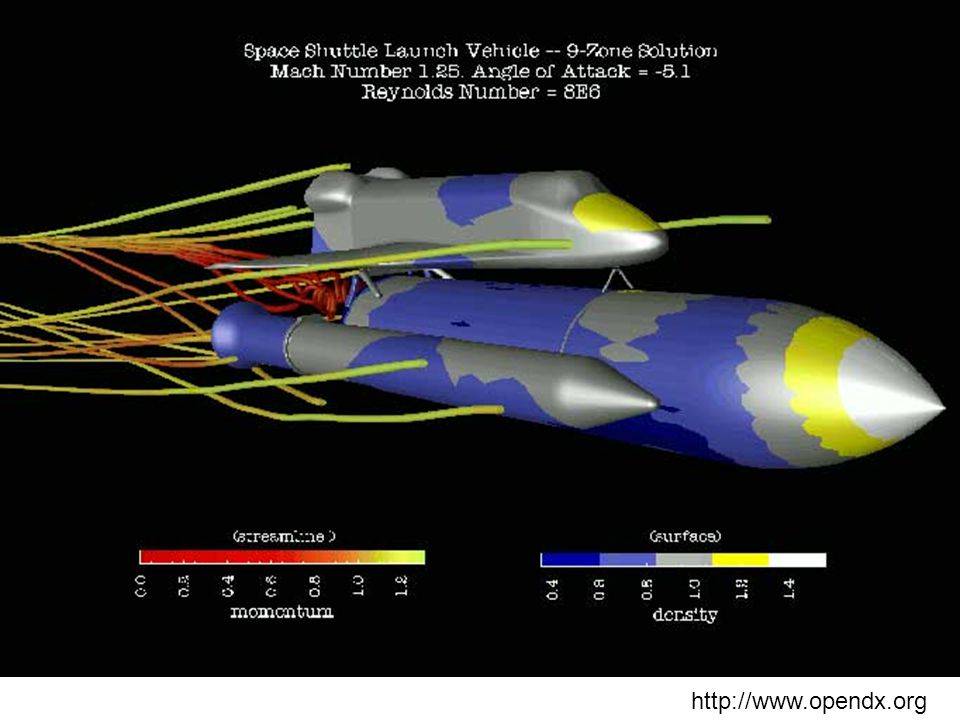
3. This image shows a single time step from an unsteady flow simulation over the Space Shuttle Launch Vehicle during launch configuration. The momentum is shown as streamlines colored by magnitude and the density on the shuttle surface is shown as filled color- mapped contours. The flow fields are computed over nine overlapping grids with almost 950,000 points. The data are available courtesy of NASA/Ames Research Center, Moffett Field, CA

4. 3b. Viscous Flow Importance of viscous effects governed by
Re=
Boundary layer: Thin region adjacent to a solid surface where friction slows the flow.
There is no pressure gradient across a boundary layer
No-slip condition: Fluid immediately adjacent to a solid surface does not move relative to it

5. 3b Viscous Flow Viscous region not always confined to a thin layer
Separation: Large region of viscous flow produced when the boundary layer leaves a surface because of an adverse pressure gradient, or a sharp corner

6. 3c. Compressibility Incompressible Regime M<0.3
Importance of compressibility effects governed by
Incompressible Regime M<0.3
Negligible compressibility effects
Subsonic Regime 0.3<M<0.7
Quantitative effects, no qualitative effects
Transonic Regime 0.7<M<1.3
Large regions of subsonic and supersonic flow. Large qualitative effects.
Supersonic Regime M>1.3
Almost entirely supersonic flow. Large qualitative effects

7. Flow Past a Circular Cylinder
Re = 10,000 and Mach approximately zero
Re = 110,000 and Mach = 0.45
Re = 1.35 M and Mach = 0.64
Pictures are from “An Album of Fluid Motion” by Van Dyke

8. Flow Past a Circular Cylinder
Mach = 0.80
Mach = 0.90
Mach = 0.95
Mach = 0.98
Pictures are from “An Album of Fluid Motion” by Van Dyke

9. Flow Past a Sphere Mach = 1.53 Mach = 4.01
Pictures are from “An Album of Fluid Motion” by Van Dyke

10. 3c. Compressibility
Some Qualitative Effects
Shock wave: Very strong, thin wave, propagating supersonically, producing almost instantaneous compression of the flow, and increase in pressure and temperature.
Hypersonic vehicle re-entry
NASA Image Library

11. 3c. Compressibility Expansion or isentropic compression wave
Some Qualitative Effects
Expansion or isentropic compression wave
Finite wave (often focused on a corner), moving at the sound speed, producing gradual compression or expansion of a flow (and raising or lowering of the temperature and pressure).
Cone-cylinder in supersonic free flight, Mach = 1.84.
Picture from “An Album of Fluid Motion” by Van Dyke.

12. Summary What a fluid is. Its properties. The governing laws
Reynolds number. Mach number
How Newton’s 2nd Law works as a vector equation
Viscous effects: no-slip condition, boundary layer, separation, wake, turbulence, laminar
Compressibility effects: Regimes, shock waves, isentropic waves.
Initial ideas of concepts such as streamlines/eddies
Qualitative understanding

13. 2. Vector Algebra

14. Vector basics Vector: A, A Magnitude: |A|, A Scalar: p,  Types
Polar vector
Velocity V, force F, pressure gradient p
Axial vector
Angular velocity , Vorticity Ω, Area A
Unit vector
i, j, k, es, n, A/A … Q
MAG
DIR P

15. Vector Algebra Addition A + B = C Dot, or scalar, product A.B = ABcos
E.g. Work=F.s
Flow rate through dA=V.dA or V.ndA
A.B=B.A A.A=A2 A.B=0 if perpendicular A C A  B

16. Vector Algebra Cross, or vector, product AxB=ABsine AxB=-BxA AxA=0
AxB=0 if A and B parallel A  B
Parallelogram area is |AxB|
Measured to be <180o
Perpendicular to A and B in direction given by RH rule rotation from A to B

17. Vector Algebra – Triple Products
(A.B)C = (B.A)C
Mixed product A.BxC
Volume of parallelepiped
bordered by A, B, C
May be cyclically permuted
A.BxC=C.AxB=B.CxA
Acyclic permutation changes
sign A.BxC=-B.AxC etc.
Vector triple product
Ax(BxC) = Vector in plane of B and C
= (A.C)B – (A.B)C B C A
BxC

18. PIV of Flow Downstream of a Circular Cylinder Chiang Shih , Florida State University

19. Cartesian Coordinates
Coordinates x, y , z
Unit vectors i, j, k (in directions of increasing coordinates) are constant
Position vector
r = x i + y j + z k
Vector components
F = Fx i+Fy j+Fz k
= (F.i) i+ (F.j) j+ (F.k) k
Components same regardless of location of vector z F k j i r z y x y x

20. Cylindrical Coordinates
Coordinates r,  , z
Unit vectors er, e, ez (in directions of increasing coordinates)
Position vector
R = r er + z ez
Vector components
F = Fr er+F e+Fz ez
Components not constant, even if vector is constant F ez e er R z  r

21. Spherical Coordinates
Errors on this slide in online presentation
Spherical Coordinates
Coordinates r,  , 
Unit vectors er, e, e (in directions of increasing coordinates)
Position vector
r = r er
Vector components
F = Fr er+F e+F e er e F r e  r 

22. Vector Algebra in Components
…works for any orthogonal coordinate system!

23. CFD of Flow Around a Fighter
FinFlo Ltd

24. Concept of Differential Change In a Vector. The Vector Field.
Scalar field
=(r,t)
Vector field
V=V(r,t) V dV
V+dV
Differential change in vector
Change in direction
Change in magnitude

25. Change in Unit Vectors – Cylindrical System
de
er+der e ez
e+de
der P' er e P z er r d 

26. Change in Unit Vectors – Spherical System r
See “Formulae for Vector Algebra and Calculus” 

27. Example Fluid particle
Differentially small piece of the fluid material
The position of fluid particle moving in a flow varies with time. Working in different coordinate systems write down expressions for the position and, by differentiation, the velocity vectors.
V=V(t)
R=R(t)
Cartesian System O
Cylindrical System
... This is an example of the calculus of vectors with respect to time.

28. Vector Calculus w.r.t. Time
Since any vector may be decomposed into scalar components, calculus w.r.t. time, only involves scalar calculus of the components