1. P M V Subbarao Professor Mechanical Engineering Department
Measurement of Flow
P M V Subbarao
Professor
Mechanical Engineering Department
An Essential Requirement in CV Based Industrial Appliances….

2. Mathematics of Flow Rate
The Scalar Product of two vectors, namely velocity and area..

3. Important characteristics of the dot product
The first point to note about the definition is that the coordinate system does not enter the definition.
The second point to note is that because cosq=cos(-q), the order is not important, that is, the scalar product is commutative.
The scalar product is also distributive.
All these qualities help in development of a single instrument to measure the scalar product.

4. Types of Flow Measurement Technologies
Variable Area (rotameters)
Rotating Vane (paddle & turbine)
Positive Displacement
Differential Pressure
Vortex Shedding
Thermal Dispersion
Magnetic Magnetic
Thermal Mass
Coriolis Mass
Ultrasonic

6. Some Facts About Variable Area Flowmeters
Called “float type float type”, “rotameter’’, or “variable area” flowmeters.
By far the most common specified, purchased, and installed flowmeter in the world

7. Variable Area Flowmeters
Fluid flow moves the float upward against gravity.
Float will find equilibrium when area around float generates enough drag equal to weight - buoyancy.
Some types have a guide rod to keep float stable.
Low Cost (pricing usually starts < $50)
Simple Reliable Design
Can Measure Liquid or Gas Flows
Tolerates Dirty Liquids or Solids in Liquid

8. Measuring Principles of Variable Area Flowmeters
Flow Rate Analysis.
The forces acting on the bob lead to equilibrium between:
the weight of the bob rbgVb acting downwards
the buoyancy force rgVb and
the drag force Fd acting upwards.
Where Vb is the volume and
rb is the density of the bob,
r is the density of the fluid, and
g is the gravitational acceleration:

9. The drag force results from the flow field surrounding the bob and particularly from the wake of the bob.
In flow analyses based on similarity principles, these influences are accounted for by empirical coefficient CL or CT in the drag law for:

10. The volume flow rate through the rotameter is:
Where m is the open area ratio, defined as:
And D is the tube diameter at the height of the bob.

12. for laminar flow:
where the parameter a is defined in terms of a constant
K =Vb/D3b characteristic of the shape of the bob:
for turbulent flow:

13. With either laminar or turbulent flow through the rotameter, the flow rate is proportional to m.
If the cross-sectional area of the tube is made to increase linearly with length, i.e.,
then since the cone angle f of the tube is small,
and the flow rate is directly proportional to the height h of the bob. h

14. Similarity Analysis.
The basic scaling parameter for flow is the Reynolds number, defined as:
where UIN is the velocity at the rotameter inlet, and the tube diameter D is represented by its value at the inlet, equal to the bob diameter Db.
Through the Reynolds number regimes of laminar or turbulent flow, and particularly important for the rotameter flow regimes with strong or weak viscosity dependence can be distinguished.
It has been found to be practical for rotameters to use an alternative characteristic number, the Ruppel number, defined as:

15. where mb = rbD3b is the mass of the bob.
By combining Equations, the mass flow through the rotameter can be written as:
The relationship between the Ruppel number and the Reynolds number:
The advantage of the Ruppel number is its independence of the flow rate.
Since the Ruppel number contains only fluid properties and the mass and the density of the bob, it is a constant for a particular instrument.

16. Design Charts for Laminar Rotameters

17. Design Charts for Turbulent Rotameters

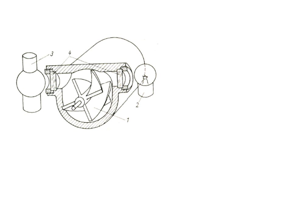
19. End fitting — flange shown;
flowmeter body;
rotation pickup — magnetic, reluctancetype shown;
permanent magnet;
pickup cold wound on pole piece;
rotor blade;
rotor hub;
Rotor shaft bearing — journal type shown;
rotor shaft;
diffuser support and flow straightener;
diffuser;
(12) flow conditioning plate (dotted) — optional with some meters.

22. Theory
There are two approaches described in the current literature for analyzing axial turbine performance.
The first approach describes the fluid driving torque in terms of momentum exchange, while the second describes it in terms of aerodynamic lift via airfoil theory.
The former approach has the advantage that it readily produces analytical results describing basic operation, some of which have not appeared via airfoil analysis.
The latter approach has the advantage that it allows more complete descriptions using fewer approximations.
However, it is mathematically intensive and leads rapidly into computer-generated solutions.

23. Eliminating the time dimension from the left-hand-side quantity reduces it to the number of rotor rotations per unit fluid volume, which is essentially the flowmeter K factor specified by most manufacturers.

24. In the ideal situation, the meter response is perfectly linear and determined only by geometry.
In some flowmeter designs, the rotor blades are helically twisted to improve efficiency.
This is especially true of blades with large radius ratios, (R/a).
If the flow velocity profile is assumed to be flat, then the blade angle in this case can be described by tan b = Constant X r.
This is sometimes called the “ideal” helical blade.
In practice, there are instead a number of rotor retarding torques of varying relative magnitudes.
Under steady flow, the rotor assumes a speed that satisfies the following equilibrium:

25. The difference between the actual rotor speed, rw, and the ideal rotor speed, rwi , is the rotor slip velocity due to the combined effect of all the rotor retarding torques , and as a result of which the fluid velocity vector is deflected through an exit or swirl angle, q.
Denoting the radius variable by r, and equating the total rate of change of angular momentum of the fluid passing through the rotor to the retarding torque, one obtains:
NT is the total retarding torque

26. Industrial Correlations for Frictional Losses

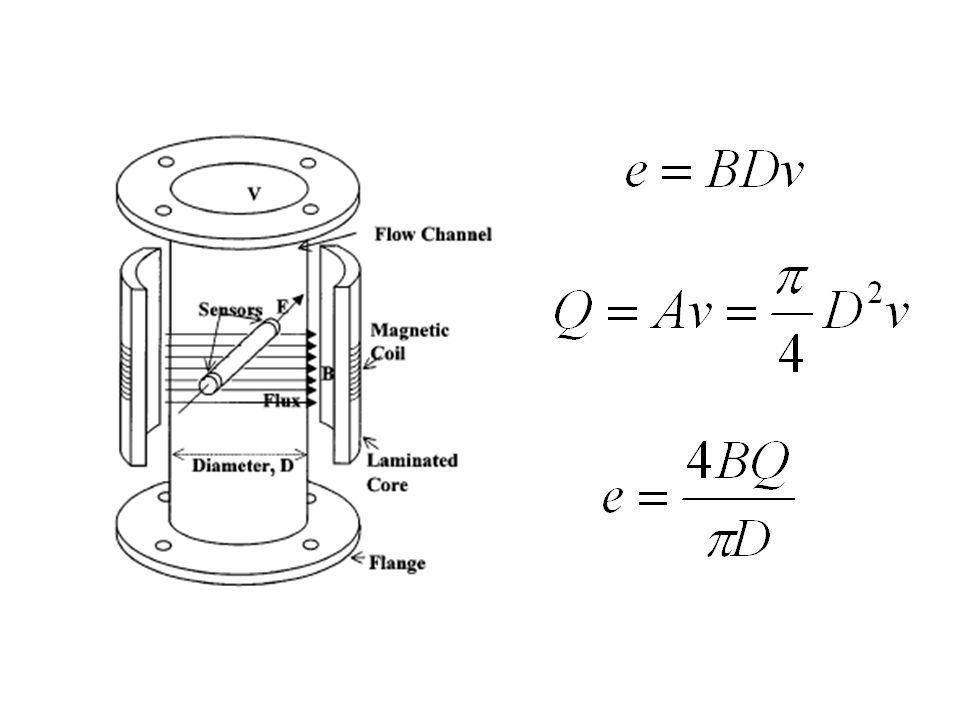
27. Electromagnetic Flowmeters
Magnetic flowmeters have been widely used in industry for many years.
Unlike many other types of flowmeters, they offer true noninvasive measurements.
They are easy to install and use to the extent that existing pipes in a process can be turned into meters simply by adding external electrodes and suitable magnets.
They can measure reverse flows and are insensitive to viscosity, density, and flow disturbances.
Electromagnetic flowmeters can rapidly respond to flow changes and they are linear devices for a wide range of measurements.
As in the case of many electric devices, the underlying principle of the electromagnetic flowmeter is Faraday’s law of electromagnetic induction.
The induced voltages in an electromagnetic flowmeter are linearly proportional to the mean velocity of liquids or to the volumetric flow rates.

28. As is the case in many applications, if the pipe walls are made from nonconducting elements, then the induced voltage is independent of the properties of the fluid.
The accuracy of these meters can be as low as 0.25% and, in most applications, an accuracy of 1% is used.
At worst, 5% accuracy is obtained in some difficult applications where impurities of liquids and the contact resistances of the electrodes are inferior as in the case of low-purity sodium liquid solutions.
Faraday’s Law of Induction
This law states that if a conductor of length l (m) is moving with a velocity v (m/s–1), perpendicular to a magnetic field of flux density B (Tesla), then the induced voltage e across the ends of conductor can be expressed by:

29. The velocity of the conductor is proportional to the mean flow velocity of the liquid.
Hence, the induced voltage becomes:

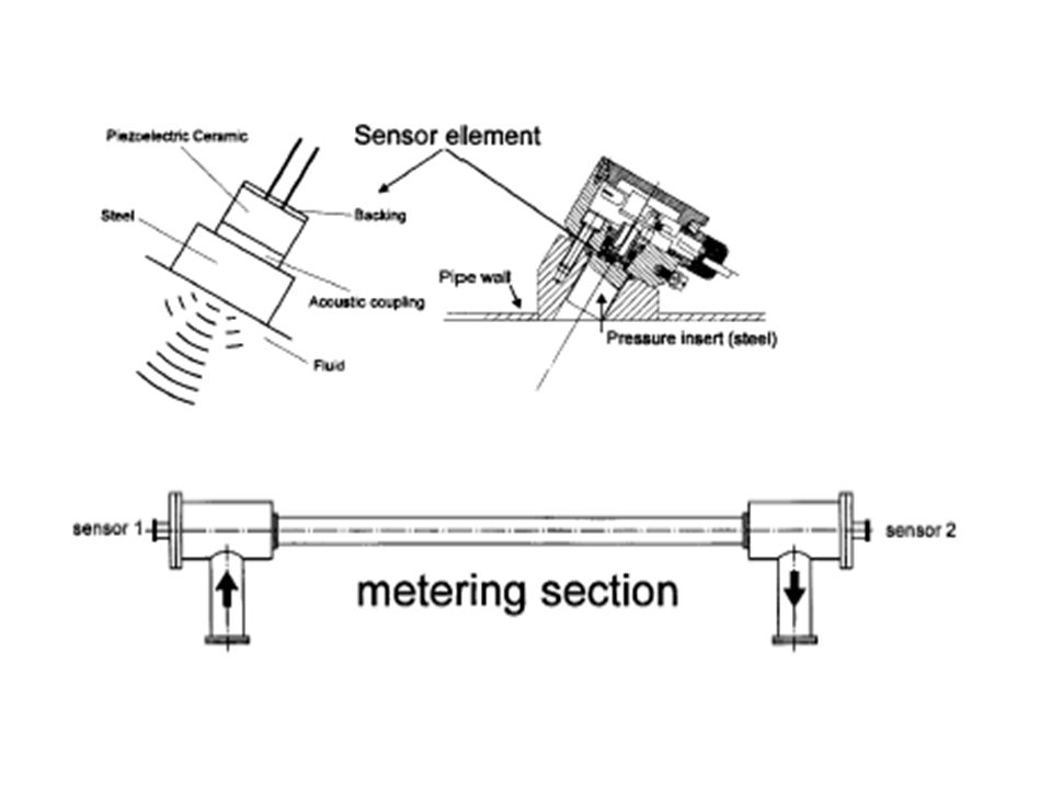
32. Ultrasonic Flowmeters
There are various types of ultrasonic flowmeters in use for discharge measurement:
(1) Transit time: This is today’s state-of-the-art technology and most widely used type.
This type of ultrasonic flowmeter makes use of the difference in the time for a sonic pulse to travel a fixed distance.
First against the flow and then in the direction of flow.
Transmit time flowmeters are sensitive to suspended solids or air bubbles in the fluid.
(2) Doppler: This type is more popular and less expensive, but is not considered as accurate as the transit time flowmeter.
It makes use of the Doppler frequency shift caused by sound reflected or scattered from suspensions in the flow path and is therefore more complementary than competitive to transit time flowmeters.

33. Principle of transit time flowmeters.

34. Transit Time Flowmeter
Principle of Operation
The acoustic method of discharge measurement is based on the fact that the propagation velocity of an acoustic wave and the flow velocity are summed vectorially.
This type of flowmeter measures the difference in transit times between two ultrasonic pulses transmitted upstream t21 and downstream t12 across the flow.
If there are no transverse flow components in the conduit, these two transmit times of acoustic pulses are given by:

35. Since the transducers are generally used both as transmitters and receivers, the difference in travel time can be determined with the same pair of transducers.
Thus, the mean axial velocity along the path is given by:

36. Example
The following example shows the demands on the time measurement technique:
Assume a closed conduit with diameter D = 150 mm, angle f = 60°, flow velocity = 1 m/s, and water temperature =20°C.
This results in transmit times of about 116 s and a time difference
Dt =t12 – t21 on the order of 78 ns.
To achieve an accuracy of 1% of the corresponding full-scale range, Dt has to be measured with a resolution of at least 100 ps (1X10–10s).
Standard time measurement techniques are not able to meet such requirements so that special techniques must be applied.
Digital timers with the state-of-the –art Micro computers will make it possible to measure these time difference.

38. Point Velocity Measurement
Pitot Probe Anemometry : Potential Flow Theory & Bernoulli’s Theory .
Thermal Anemometry : Newton’s Law of Cooling.
Laser Anemometry: Doppler Theory.