1. Linear and Nonlinear Modeling Class web site: http://statwww.epfl.ch/davison/teaching/Microarrays/ Statistics for Microarrays

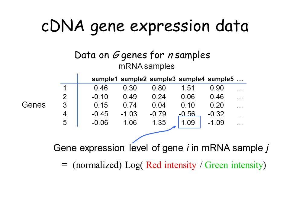
2. cDNA gene expression data Data on G genes for n samples Genes mRNA samples Gene expression level of gene i in mRNA sample j = (normalized) Log( Red intensity / Green intensity) sample1sample2sample3sample4sample5 … 1 0.46 0.30 0.80 1.51 0.90... 2-0.10 0.49 0.24 0.06 0.46... 3 0.15 0.74 0.04 0.10 0.20... 4-0.45-1.03-0.79-0.56-0.32... 5-0.06 1.06 1.35 1.09-1.09...

3. Identifying Differentially Expressed Genes Goal: Identify genes associated with covariate or response of interest Examples: –Qualitative covariates or factors: treatment, cell type, tumor class –Quantitative covariate: dose, time –Responses: survival, cholesterol level –Any combination of these!

4. Modeling Introduction Want to capture important features of the relationship between a (set of) variable(s) and one or more responses Many models are of the form g(Y) = f(x) + error Differences in the form of g, f and distributional assumptions about the error term

5. Examples of Models Linear: Y =  0 +  1 x +  Linear: Y =  0 +  1 x +  2 x 2 +  (Intrinsically) Nonlinear: Y =  x 1  x 2  x 3  +  Generalized Linear Model (e.g. Binomial): ln(p/[1-p]) =  0 +  1 x 1 +  2 x 2 Proportional Hazards (in Survival Analysis): h(t) = h 0 (t) exp(  x)

6. Linear Modeling A simple linear model: E(Y) =  0 +  1 x Gaussian measurement model: Y =  0 +  1 x + , where  ~ N(0,  2 ) More generally: Y = X  + , where Y is n x 1, X is n x G,  is G x 1,  is n x 1, often assumed N(0,  2 I nxn )

7. Analysis of Designed Experiments An important use of linear models Here, the response (Y) is the gene expression level Define a (design) matrix X so that E(Y) = X , where  is a vector of contrasts Many ways to define design matrix/contrasts

8. Contrasts (I) Example: One-way layout, k classes Y ij =  +  j +  ij, i = 1,…,n j ; j = 1,…,k X = 1 1 0 … 0 = [1 X a ] 1 0 1 … 0 … 1 0 0 … 1 Problem: this specification is over- parametrized

9. Contrasts (II) Could resolve by removing column of 1’s: Y ij =  j +  ij, i = 1,…,n j ; j = 1,…,k X = 1 0 … 0 = [X a ] 0 1 … 0 … 0 0 … 1 Here, parameters are class means

10. Contrasts (III) Define design matrix X * = [1 X a C a ], with C a (k x (k-1)) chosen so that X * has rank k (the number of columns) Parameters may become difficult to interpret In the balanced case (equal number of observations in each class), can choose orthogonal contrasts (Helmert)

11. Model Fitting For the standard (fixed effects) linear model, estimation is usually by least squares Can be more complicated with random effects or when x-variables subject to measurement error as well (so that estimates are not biased)

12. Model Checking Examination of residuals –Normality –Time effects –Nonconstant variance –Curvature Detection of influential observations

13. Do we need robust methods? Tukey (1962): “A tacit hope in ignoring deviations from ideal models was that they would not matter; that statistical procedures which were optimal under the strict model would still be approximately optimal under the approximate model. Unfortunately it turned out that this hope was often drastically wrong; even mild deviations often have much larger effects than were anticipated by most statisticians.”

14. Robust Regression Idea: downweight observations that produce large residuals More computationally intensive than least squares regression (which gives equal weight to each observation) Use maximum likelihood if can assume specific error distribution When not, use M-estimators

15. M-estimators ‘Maximum likelihood type’ estimators Assume independent errors with distribution f(  ) Robust estimator minimizes  i  (e i /s) =  i  {(Y i – x i ’  )/s}, where  (.) is some function and s is an estimate of scale  (u) = u 2 corresponds to minimizing the sum of squares

16. M-estimation Procedure To minimize  i  {(Y i – x i ’  )/s} wrt the  ’s, take derivatives and equate to 0 Resulting equations do not have an explicit solution in general Solve by iteratively reweighted least squares

17. Examples of Weight Functions

18. Generalized Linear Models (GLM/GLIM) Response Y assumed to have exponential family distribution: f(y) = exp[a(y)b(  ) + c(  ) + d(y)] Parameters  and explanatory variables X; linear predictor  =  1 x 1 +  2 x 2 + …  p x p Mean response , link function l (  ) =  Allows unified treatment of statistical methods for several important classes of models

19. Some Examples LinkBinomialGammaNormalPoisson logit Default probit X cloglog X identity XXX inverse Default Log XDefault Sqrt X

20. (BREAK)

21. Survival Modeling Response T is a (nonnegative) lifetime Cumulative distribution function (cdf) F(t), density f(t) More usual to work with the survivor function S(t) = 1 – F(t) = P(T > t) and the instantaneous failure rate, or hazard function h(t) = lim  t->0 P(t  T< t+  t | T  t)/  t

22. Relations Between Functions Cumulative hazard function H(t) =  0 t h(s) ds h(t) = f(t)/S(t) H(t) = -log S(t)

23. Censoring Incomplete information on the lifetime A censored observation is one whose value is incomplete due to random factors for each individual Most commonly, observation begins at time t = 0 and ends before the outcome of interest is observed (right-censoring)

24. Estimation of Survivor Function Most commonly used estimate is Kaplan-Meier (also called product limit) estimator Risk set r(t) = number of cases alive just before time t S(t) =  t i  t [r(t i ) – d i ]/r(t i ) ^

25. Cox Proportional Hazards Model Baseline hazard function h 0 (t) Modified multiplicatively by covariates Hazard function for individual case is h(t) = h 0 (t) exp(  1 x 1 +  2 x 2 + … +  p x p ) If nonproportionality: –1. Does it matter –2. Is it real

26. Strategies for Gene Expression-based Modeling The biggest problem is the large number of variables (genes) One possibility is to first reduce the number of genes under consideration (e.g. consider variability across samples, or coefficient of variation) Screening/Prioritizing: One gene at a time approach Two at a time, perhaps plus interaction

27. Example: Survival analysis with expression data Bittner et al. dataset: –15 of the 31 melanomas had associated survival times –3613 ‘strongly detected’ genes

28. ‘cluster’ unclustered Average Linkage Hierarchical Clustering

29. Association of Variables Variables tested for association with cluster: –Sex (p =.68, n = 16 + 11 = 27)  Age (p =.14, n = 15 + 10 = 25)  Mutation status (p =.17, n = 12 + 7 = 19) –Biopsy site (p =.88, n = 14 + 10 = 24) –Pigment (p =.26, n = 13 + 9 = 22) –Breslow thickness (p =.26, n = 6 + 3 = 9) –Clark level (p =.44, n = 6 + 5 = 11)  Specimen type (p =.11, n = 11 + 12 = 23)

30. Survival analysis: Bittner et al. Bittner et al. also looked at differences in survival between the two groups (the ‘cluster’ and the ‘unclustered’ samples) ‘Cluster’ seemed associated with longer survival

31. Kaplan-Meier Survival Curves

32. unclustered cluster Average Linkage Hierarchical Clustering, survival samples only

33. Kaplan-Meier Survival Curves, new grouping

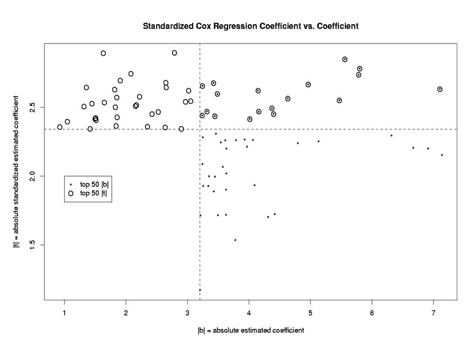
34. Identification of Genes Associated with Survival For each gene j, j = 1, …, 3613, model the instantaneous failure rate, or hazard function, h(t) with the Cox proportional hazards model: h(t) = h 0 (t) exp(  j x ij ) and look for genes with both: large effect size  j large standardized effect size  j /SE(  j ) ^ ^^

36. Sites Potentially Influencing Survival Image Clone ID UniGene Cluster UniGene Cluster Title 137209Hs.126076Glutamate receptor interacting protein 240367Hs.57419Transcriptional repressor 838568Hs.74649Cytochrome c oxidase subunit Vlc 825470Hs.247165ESTs, Highly similar to topoisomerase 841501Hs.77665KIAA0102 gene product

37. Findings Top 5 genes by this method not in Bittner et al. ‘weighted gene list’ - Why? weighted gene list based on entire sample; our method only used half weighting relies on Bittner et al. cluster assignment other possibilities?

38. Statistical Significance of Cox Model Coefficients

39. Advantages of Modeling Can address questions of interest directly –Contrast with what has become the ‘usual’ (and indirect) approach with microarrays: clustering, followed by tests of association between cluster group and variables of interest Great deal of existing machinery Quantitatively assess strength of evidence

40. Limitations of Single Gene Tests May be too noisy in general to show much Do not reveal coordinated effects of positively correlated genes Hard to relate to pathways

41. Not Covered… Careful followup –Assessment of proportionality –Inclusion of combinations of genes, interactions –Consideration of alternative models Power assessment –Not worth it here, there can’t be much!

42. Some ideas for further work Expand models to include more genes, possibly two-way interactions –Issue of automation –Still very small scale compared to probable pathway size, number of genes involved, etc. Nonparametric tree-based modeling –Will require much larger sample sizes

43. Acknowledgements Debashis Ghosh Erin Conlon Sandrine Dudoit José Correa