1. Chapter 3 Simple Regression

2. What is in this Chapter? This chapter starts with a linear regression model with one explanatory variable, and states the assumptions of this basic model It then discusses two methods of estimation: the method of moments and the method of least squares. The method of maximum likelihood is discussed in the appendix

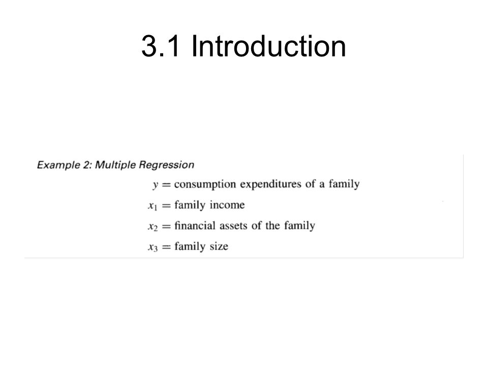
3. 3.1 Introduction

5. There are several objectives in studying these relationships. They can be used to: –1. Analyze the effects of policies that involve changing the individual x's. In Example 1 this involves analyzing the effect of changing advertising expenditures on sales –2. Forecast the value of y for a given set of x's. –3. Examine whether any of the x's have a significant effect on y.

6. 3.1 Introduction Given the way we have set up the problem until now, the variable y and the x variables are not on the same footing Implicitly we have assumed that the jc's are variables that influence y or are variables that we can control or change and y is the effect variable. There are several alternative terms used in the literature for y and x1, x2,..., xk. These are shown in Table 3.1.

7. 3.1 Introduction

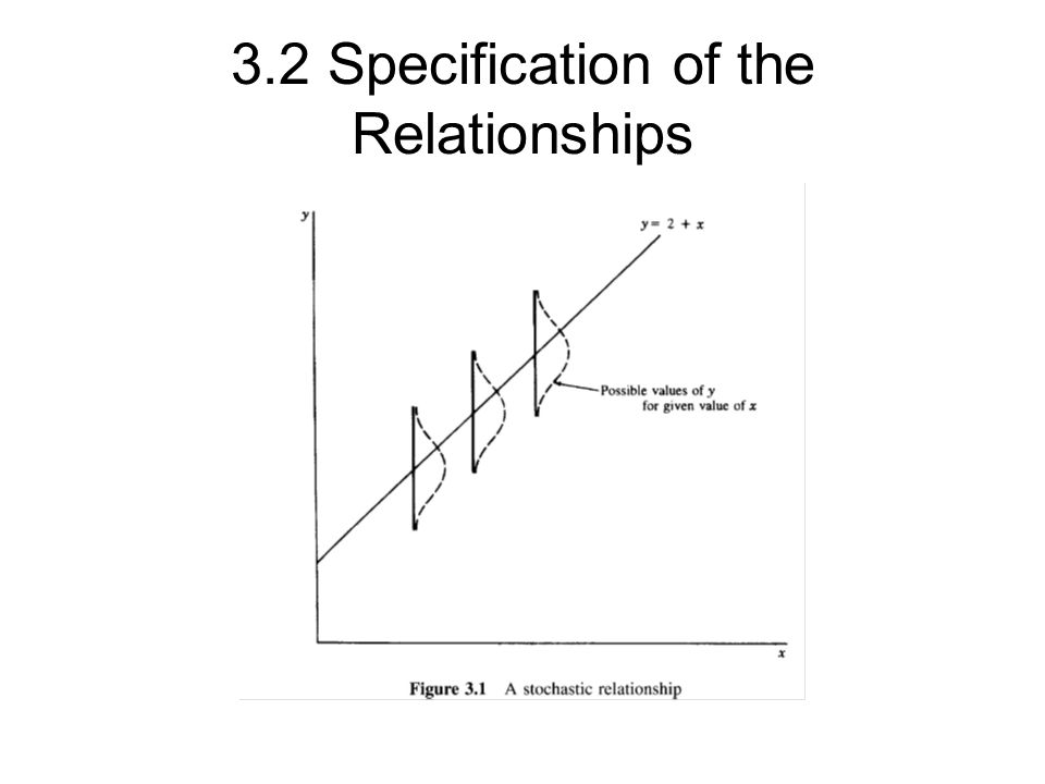
8. 3.2 Specification of the Relationships

11. In equation (3.2), α + βx is the deterministic component of y and u is the stochastic or random component. α and β are called regression coefficients or regression parameters that we estimate from the data on y and x

12. 3.2 Specification of the Relationships Why should we add an error term u7 What are the sources of the error term u in equation (3.2)? There are three main sources: –1. Unpredictable element of randomness in human responses. For instance, if y =consumption expenditure of a household and x = disposable income of the household, there is an unpredictable element of randomness in each household's consumption. The household does not behave like a machine. In one month the people in the household are on a spending spree. In another month they are tightfisted.

13. 3.2 Specification of the Relationships –2. Effect of a large number of omitted variables. Again in our example x is not the only variable influencing y. The family size, tastes of the family, spending habits, and so on, affect the variable y. The error u is a catchall for the effects of all these variables, some of which may not even be quantifiable, and some of which may not even be identifiable. To a certain extent some of these variables are those that we refer to in source 1.

14. 3.2 Specification of the Relationships –3. Measurement error in y. In our example this refers to measurement error in the household consumption. That is, we cannot measure it accurately. This argument for u is somewhat difficult to justify, particularly if we say that there is no measurement error in x (household disposable income). The case where both y and x are measured with error is discussed in Chapter 11. Since we have to go step by step and not introduce all the complications initially, we will accept this argument; that is, there is a measurement error in y but not in x.

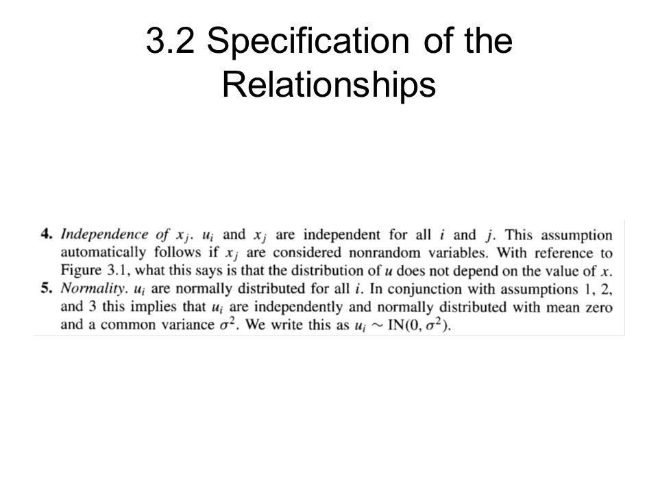
15. 3.2 Specification of the Relationships

17. These are the assumptions with which we start. We will, however, relax some of these assumptions in later chapters. Assumption 2 is relaxed in Chapter 5. Assumption 3 is relaxed in Chapter 6. Assumption 4 is relaxed in Chapter 9.

18. 3.2 Specification of the Relationships We will discuss three methods for estimating the parameters α and β: 1. The method of moments. 2. The method of least squares. 3. The method of maximum likelihood.

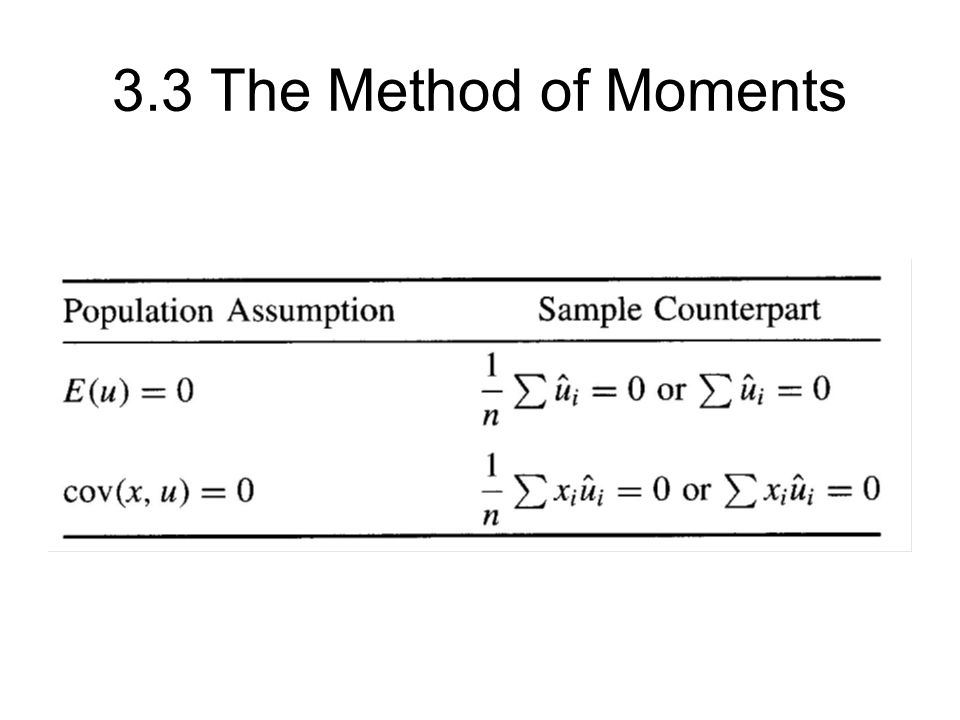
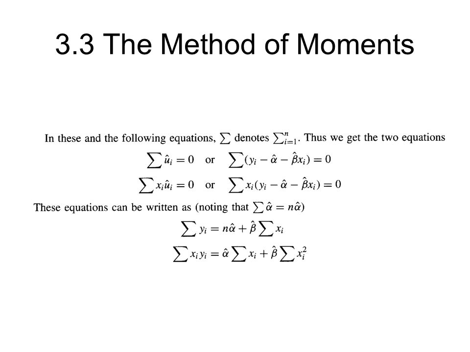
19. 3.3 The Method of Moments

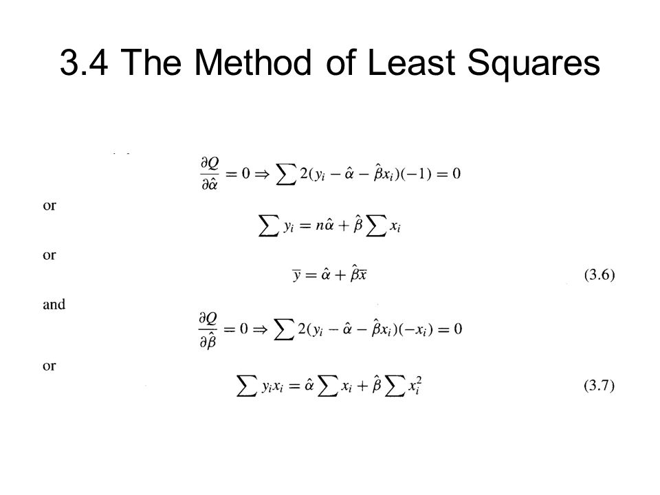
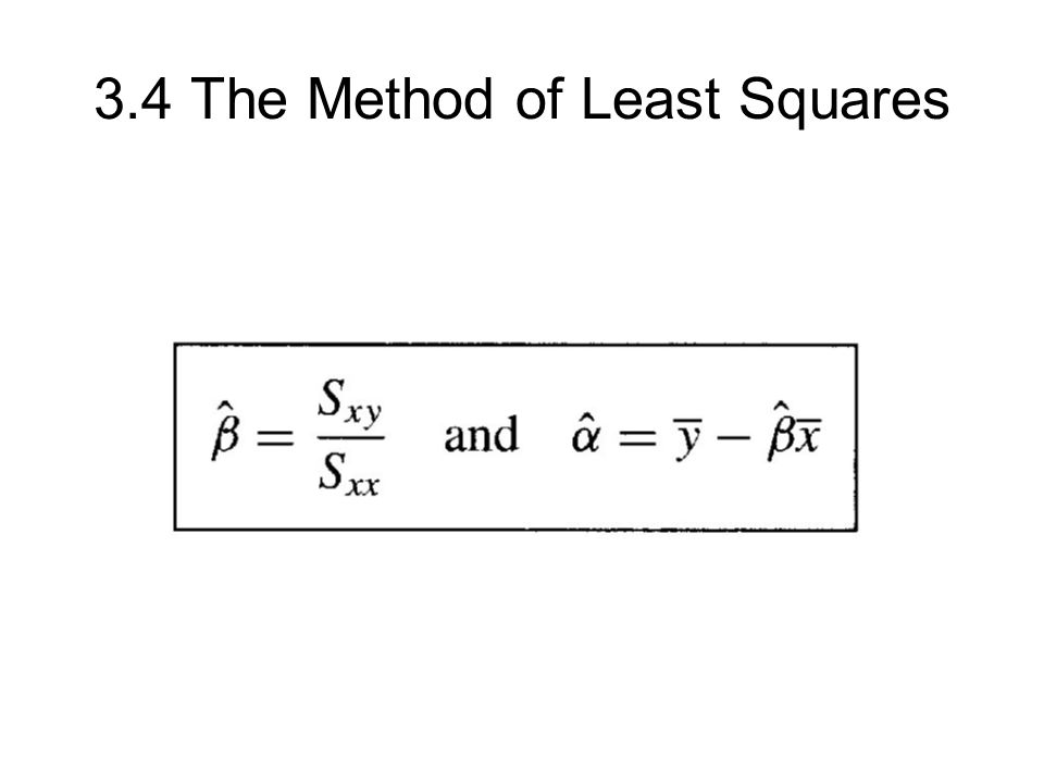
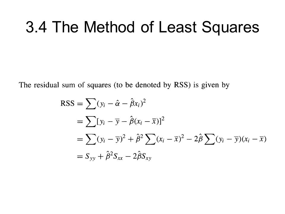
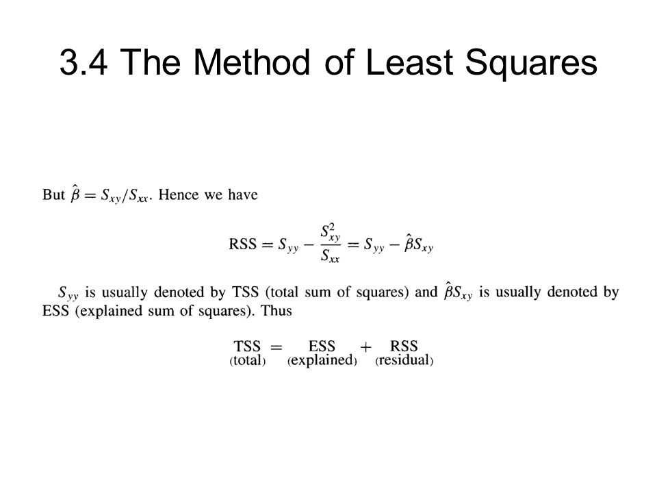
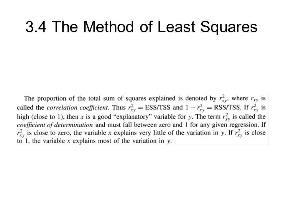
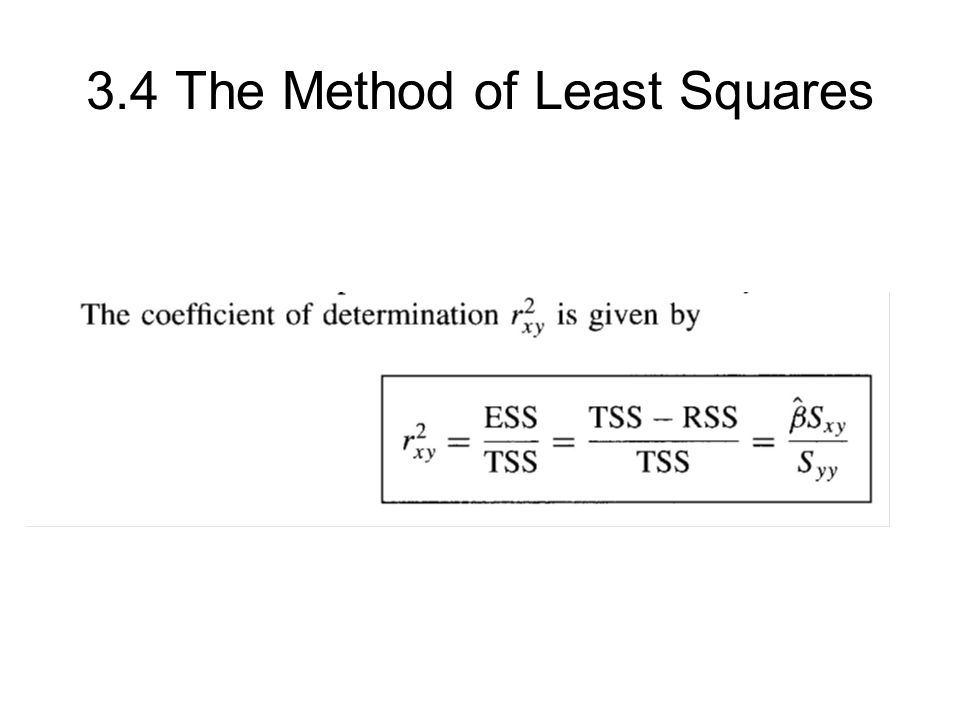
22. 3.4 The Method of Least Squares

30. Appendix to Chapter 3 Proof that the OLS estimators are BLUE The method of maximum likelihood

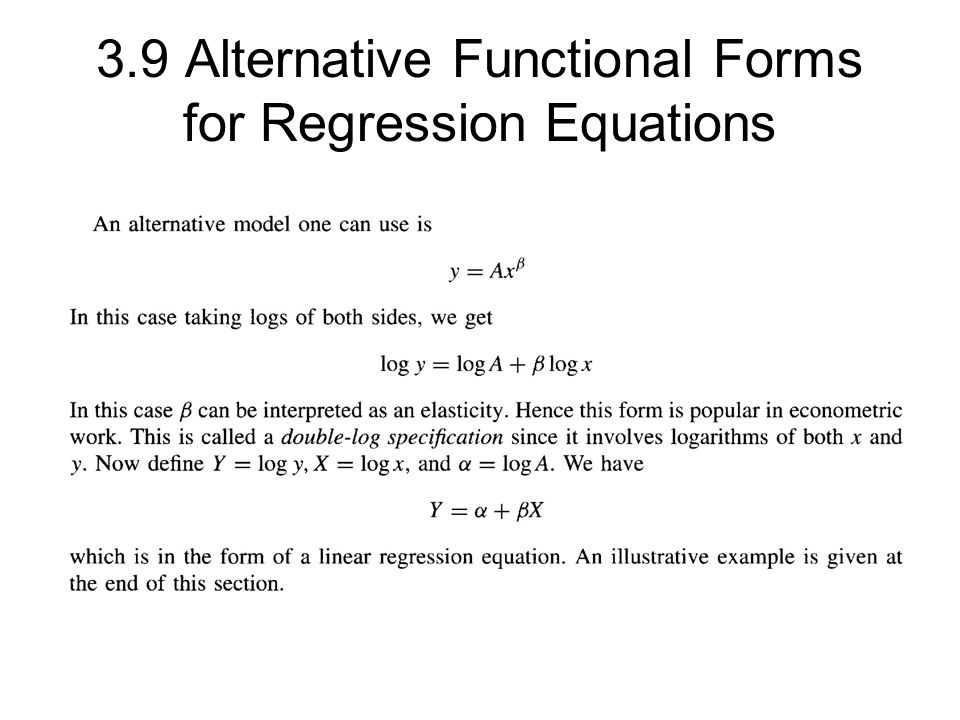
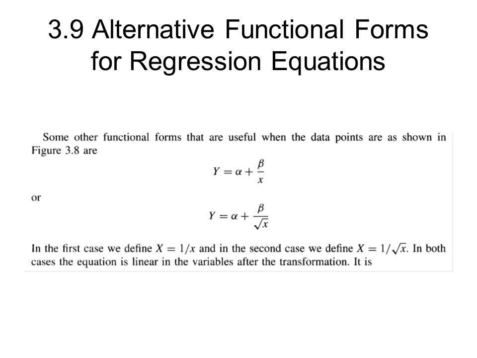
31. 3.9 Alternative Functional Forms for Regression Equations For instance, for the data points depicted in Figure 3.7(a), where y is increasing more slowly than x, a possible functional form is y = α +βlogx. This is called a semilog form, since it involves the logarithm of only one of the two variables x and y. In this case, if we redefine a variable X = logx, the equation becomes y = α + βX. Thus we have a linear regression model with the explained variable y and the explanatory variable X = logx

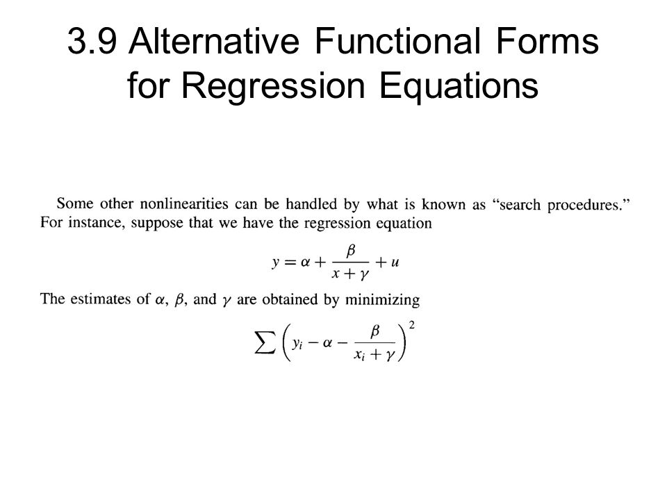
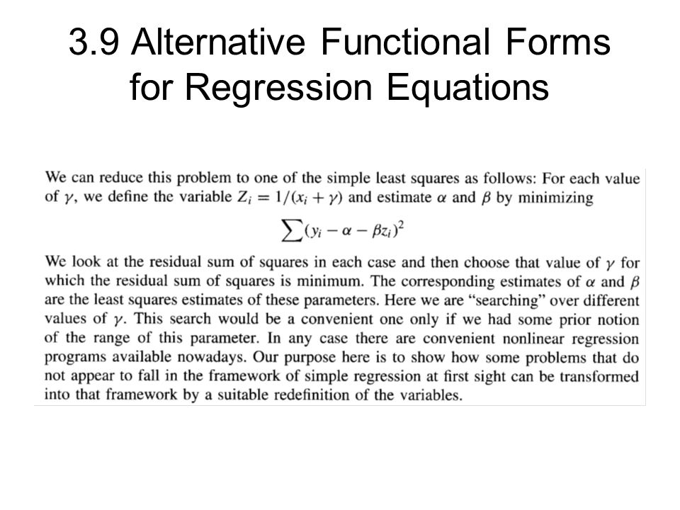
32. 3.9 Alternative Functional Forms for Regression Equations