1. Study of Sparse Online Gaussian Process for Regression EE645 Final Project May 2005 Eric Saint Georges

2. A.Introduction B.OGP 1.Definition of Gaussian Process 2.Sparse Online GP algorithm (OGP) C.Simulation Results 1.Comparison with LS SVM on Boston Housing data set (Batch) 2.Time Series Prediction using OGP 3.Optical Beam Position Optimization D.Conclusion Contents

3. Introduction Possible Application of OGP to Optical Free Space Communication for Monitoring and Optimization in a noisy environment Using Sparse OGP Algorithm developed by Lehel Csato and al.

4. A.Introduction B.OGP 1.Definition of Gaussian Process 2.Sparse Online GP algorithm (OGP) C.Simulation Results 1.Comparison with LS SVM on Boston Housing data set (Batch) 2.Time Series Prediction using OGP 3.Optical Beam Position Optimization D.Conclusion Contents

5. Gaussian Process Definition Collection of indexed random variables –Mean –Covariance defined by a Kernel function function: can be any Positive Semi Definite function Defines the assumptions on the prior distribution Wide scope of choices Popular Kernels are stationary functions: f (x-x’) –Index can be time or space or anything else

6. On line GP Process Bayesian Process: Prior distribution (GP Process) + Likelihood Function Posterior distribution (Using Bayes rule)

7. Solving a Gaussian Process: Given measures n inputs and n measures t i (with t i = y i + e i ) being zero mean and  e variance Prior distribution over y i is given by the covariance matrix K ij = C(x i,x j ). Prior distribution over the measures t i is given by K+  e I n Prediction on function y * for an input x * consists in calculating the mean and variances: y * (x * )=  i C(x i,x j ) and  (x * )=C(x *,x * ) –k T (x * )(K +  e I n ) -1 k (x * ) With  i = (K +  e I n ) -1 t

8. Solving the Gaussian Process: Solving requires inversion of (K +  e I n ) which is a n x n matrix, n being the number of training inputs. Memory is in n 2 and cpu time in n 3.

9. Sampling from a Gaussian Process: Example of Kernel: a = amplitude s = scale (smoothness)

10. Sampling from a GP: before Training

11. Effect of Scale Small Scale=1 Large Scale =100

12. Sampling from a GP: before Training Effect of Scale Small Scale=1 Large Scale =100

13. Sampling from a GP: After Training After 3 Training samples

14. Sampling from a GP: After Training After 10 Training samples

15. Online Gaussian Process: Issues Two Major Issues with the GP process; 1.Data Set size is limited by Memory and CPU 2.Posterior distribution is usually not Gaussian

16. Algorithm developed by Csato and al. Sparse Online Gaussian Algorithm Sparsity created using limited number of SVs Gaussian Approximation Posterior Distribution Not usually Gaussian Data Set size limited by Memory and CPU Matlab Software available on the Web

17. SOGP Process defined by: –Kernel Parameters m + 2 Vector for RBF Kernel –Support Vectors: d x 1 Vector (indexes) –GP Parameters:  : d x 1 Vector K:d x n Matrix m dimension of input space d number of support vectors Sparse Online Gaussian Algorithm

18. A.Introduction B.OGP 1.Definition of Gaussian Process 2.Sparse Online GP algorithm (SOGP) C.Simulation Results 1.Comparison with LS SVM on Boston Housing data set (Batch) 2.Time Series Prediction using OGP 3.Optical Beam Position Optimization D.Conclusion

19. LS SVM on Boston Housing Data Set RBF Kernel C=10,  =4 304 training samples averaged on 10 Random draws Average cpu = 3 sec / run

20. Kernel : Initial Hyper-parameters: and (i=1 to 13 for BH) Number of Hyper-parameter optimization iterations: tried between 3 and 6 Max number of Support Vectors: Variable OGP on Boston Housing Data Set

21. 6 Iterations, MaxBV between 10 and 250 OGP on Boston Housing Data Set

22. 3 Iterations, MaxBV between 10 and 150 OGP on Boston Housing Data Set

23. 4 Iterations, MaxBV between 10 and 150 OGP on Boston Housing Data Set

24. 6 Iterations, MaxBV between 10 and 150 OGP on Boston Housing Data Set

25. Cpu Time a*(b+SVs 2 )/SVs as a function of SVs OGP on Boston Housing Data Set

26. Run with 4 Iterations, MaxBV between 10 and 60 OGP on Boston Housing Data Set

27. Final Run with 4 Iterations, MaxBV 30 and 40 Average over 50 random draws OGP on Boston Housing Data Set

28. MSE not as good as LS SVM (6.9 versus to 6.5) But Standard deviation better than LS SVM (1.1 versus 1.6). Cpu Time much longer (90sec versus 3 sec per run) But increases slower with number of samples than LS SVM. Might do better with large data sets. Conclusion OGP on Boston Housing Data Set

29. TSP (Time Series Prediction) OGP on TSP

30. OGP on TSP: Initial Runs

33. OGP on TSP: Local Minimum For both runs: Initial kpar = 1e-2 Final kpar = 1.42e-2 MSE = 1132 Final kpar = 2.45e-3 MSE = 95

34. OGP on TSP: Impact of Over-fitting

35. OGP on TSP: Impact of Number of Samples on Prediction

36. cpu=6sec

37. OGP on TSP: Impact of Number of Samples on Prediction cpu=16 sec

38. OGP on TSP: Impact of Number of Samples on Prediction cpu=27sec

39. OGP on TSP: Impact of Number of Samples on Prediction cpu=45sec

40. OGP on TSP: Impact of Number of Samples on Prediction cpu=109sec

41. OGP on TSP: Impact of Number of Samples on Prediction cpu=233sec

42. OGP on TSP: Impact of Number SVs on Prediction

43. cpu=19sec

44. OGP on TSP: Impact of Number SVs on Prediction cpu=16sec

45. OGP on TSP: Impact of Number SVs on Prediction cpu=16sec

46. OGP on TSP: Final Runs

47. Running 200 Sample at a time, with 30 sample overlap OGP on TSP: Final Runs

48. OGP on TSP: Why an overlap?

49. Does not always behaves!... OGP on TSP: Final Runs

50. Difficult to find the right set of parameters Initial Kernel Parameter Number of Support Vectors Number of Training Samples per run OGP on TSP: Conclusion

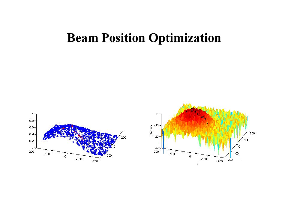
51. Beam Position Optimization

52. Gaussian Beam With Small Noise

53. Gaussian Beam With Noise

54. Gaussian Beam With Noise

55. Gaussian Beam With Noise

56. Gaussian Beam With Noise

57. Gaussian Beam Position Optimization Sampling the beam at a given position, and measuring Power Objective: Find the top of the beam

58. Idea: –With a few initial samples, use the OGP to get an estimate of the beam profile and position –Move toward the max of the estimate –Add this new sample to the training set –Iterate Beam Position Optimization

72. Works faster than current algorithm (Finds the top with less steps) Does not work well if no noise. Can be improved OGP for Beam Optimization: Conclusion

73. Specific Kernel: s1 = s2 (Beam is symmetric in x, y) Use the known Beam divergence to set the initial Kernel Parameters Optimize choice of sample –Going directly to the estimated top might not be the best (Because it does not help to improve the estimate) –Improve robustness by minimizing probability to sample at lower power OGP for Beam Optimization: Possible Improvements

74. A.Introduction B.OGP 1.Definition of Gaussian Process 2.Sparse Online GP algorithm (OGP) C.Simulation Results 1.Comparison with LS SVM on Boston Housing data set (Batch) 2.Time Series Prediction using OGP 3.Optical Beam Position Optimization D.Conclusion

75. OGP is an interesting tool Complex software Many tunings to insure stability and convergence Not easy to use Next Steps: More comparison with online LS SVM –Performance –Cpu Time Conclusion

76. References [1] Gaussian Processes, C.K. Williams, March1, 2002 [2] Efficient Implementation of Gaussian Processes, Mark Gibbs, David J.C. MacKay, May 28, 1997 [3]Sparse Online Gaussian Processes, Lehel Csató, Manfred Opper, October 9, 2002 [4]Neural Networks for pattern Recognition, Christopher M. Bishop [5]Time Series Competition Data downloaded from http://www.esat.kuleuven.ac.be/sista/workshop/competition.html http://www.esat.kuleuven.ac.be/sista/workshop/competition.html [6]Castó OGP toolbox for Matlab and Demo Program Tutorial from http://www.kyb.tuebingen.mpg.de/bs/people/csatol/ogp /http://www.kyb.tuebingen.mpg.de/bs/people/csatol/ogp /