Download presentation
Presentation is loading. Please wait.

1
Exposure In Wireless Ad-Hoc Sensor Networks S. Megerian, F. Koushanfar, G. Qu, G. Veltri, M. Potkonjak ACM SIG MOBILE 2001 (Mobicom) Journal version: S. Megerian, F. Koushanfar, G. Qu, G. Veltri, M. Potkonjak. “Exposure In Wireless Sensor Networks: Theory And Practical Solutions.” ACM Journal of Wireless Networks, 8 (5): pp. 443-454, September 2002.
 Journal version: S. Megerian, F. Koushanfar, G. Qu, G. Veltri, M. Potkonjak. Exposure In Wireless Sensor Networks: Theory And Practical Solutions. ACM Journal of Wireless Networks, 8 (5): pp , September")
2
Outline Introduction Preliminaries Minimal Exposure Path General Exposure Computations Experimental Results

3
Introduction(1/4) Coverage in sensor networks How well do the sensors observe physical space?” A measure of quality of service (surveillance) that can be provided by a particular sensor network.
 Coverage in sensor networks How well do the sensors observe physical space A measure of quality of service (surveillance) that can be provided by a particular sensor network.")
4
Introduction(2/4) Coverage Types Area coverage The main objective is to cover (monitor) an area Such as Node self-scheduling algorithm, Probing- based density control algorithm and Disjoint dominating sets heuristic, etc. Ref. [http://vc.cs.nthu.edu.tw/home/paper/list.php]

5
Introduction(3/4) Point coverage The objective is to cover a set of targets (points) Such as Disjoint set cover heuristics (Linear programming-based approaches) Ref. [http://vc.cs.nthu.edu.tw/ezLMS/show.php?id=376&1155473386] target

6
Introduction(4/4) Barrier Coverage The goal is to minimize the probability of undetected penetration through the barrier (sensor network) Maximal breach path, maximal support path, minimal exposure path. Maximal breach path Ref. [http://vc.cs.nthu.edu.tw/ezLMS/show.php?id=326&1155473548]

7
Preliminaries Sensor Models Sensing ability diminishes as distance increases Sensing ability improves as the allotted sensing time (exposure) increases Sensor field intensity All-sensor field intensity Sensing measure at point p from all sensors in F Closest-sensor field intensity Sensing measure at point p from the closest sensor in F
 increases Sensor field intensity All-sensor field intensity Sensing measure at point p from all sensors in F Closest-sensor field intensity Sensing measure at point p from the closest sensor in F")
8
Exposure Expected average ability of observing a target in the sensor field The exposure of an object moving in the sensor field during the interval [ t 1, t 2 ] along the path p(t) is defined as r rr
![Exposure Expected average ability of observing a target in the sensor field The exposure of an object moving in the sensor field during the interval [ t 1, t 2 ] along the path p(t) is defined as r rr](http://images.slideplayer.com/17/5353503/slides/slide_8.jpg "Exposure Expected average ability of observing a target in the sensor field The exposure of an object moving in the sensor field during the interval [ t 1, t 2 ] along the path p(t) is defined as r rr")
9
Minimal Exposure Path Given: Sensor Field A N sensors Initial and final points I and F Problem: Find the Minimal Exposure Path P minE in A, starting in I and ending in F. P minE is the path in A, along which the exposure is the smallest among all paths from I to F.

10
Examples(1/3) Square field One sensor is at position (0,0) Minimum exposure path from point p(1, 0) to point q(0, 1) s y p=(1, 0) q=(0, 1) /4
 Square field One sensor is at position (0,0) Minimum exposure path from point p(1, 0) to point q(0, 1) s y p=(1, 0) q=(0, 1) /4")
11
Examples(2/3) Square field (cont’) Minimum exposure path from point p(1, -1) to point q(-1, 1) Proof:
 Square field (cont’) Minimum exposure path from point p(1, -1) to point q(-1, 1) Proof:")
12
Examples(3/3) Convex polygon field Sensor is at the center of the inscribed circle The minimum exposure path from vertices v 2 vertices to v n
 Convex polygon field Sensor is at the center of the inscribed circle The minimum exposure path from vertices v 2 vertices to v n")
13
General Exposure Computations (1/3) Finding the minimum exposure path under arbitrary sensor and intensity model is extremely difficult Need Efficient and scalable methods To approximate exposure integrals To search for minimum exposure path Algorithm 1. Use grid-based approach 2. Transform the grid into a weighted graph 3. Use Djikstra’s Single-Source-Shortest-Path algorithm

14
General Exposure Computations (2/3) Step 1 Divide the sensor network region using an n×n grid The path is restricted to line segments connecting any two vertices. Example: 2×2 gird First-order (m=1)Second-order (m=2)Third-order (m=3)
Second-order (m=2)Third-order (m=3).")
15
General Exposure Computations (3/3) Step2 Transform F to the edge-weighted graph G Each edge is assigned a weight equal to the exposure along its corresponding edge in F Exposure is calculated using numerical integration techniques Step3 Find the minimal exposure path from source p s to the p d Use Djikstra’s Single-Source-Shortest-Path algorithm Can use Floyd-Warshal’s All-Pair-Shortest-Path algorithm to find minimal exposure path between any arbitrary starting and ending points.
 Step2 Transform F to the edge-weighted graph G Each edge is assigned a weight equal to the exposure along its corresponding edge in F Exposure is calculated using numerical integration techniques Step3 Find the minimal exposure path from source p s to the p d Use Djikstra’s Single-Source-Shortest-Path algorithm Can use Floyd-Warshal’s All-Pair-Shortest-Path algorithm to find minimal exposure path between any arbitrary starting and ending points.")
16
Experimental Results (1/4) Simulation platform C++ package Sensor field is 1000×1000 square Assume a constant speed 32 32 grid with 8 divisions per grid- square edge (n=32, m=8)
 Simulation platform C++ package Sensor field is 1000×1000 square Assume a constant speed 32 32 grid with 8 divisions per grid- square edge (n=32, m=8)")
17
(1/d 2 ) (1/d 4 ) 1.As n is small, there are a wide range of minimal exposure paths. 2. As n increases, the exposure and the minimal path tend to stabilize. The minimal exposure path gets closer to bounding edges of the field The path length approaches the half field perimeter. averagemedianstandard deviation

18
Experimental Results (2/4) Uniformly distributed random sensor deployment As sensor density increases, the minimal exposure value and path lengths tends to stabilize As number of sensor increases, relative standard deviation of exposure diminishes
 Uniformly distributed random sensor deployment As sensor density increases, the minimal exposure value and path lengths tends to stabilize As number of sensor increases, relative standard deviation of exposure diminishes")
19
Experimental Results (3/4) Uniformly distributed random sensor deployment (cont’) Path calculated by 8×8 grid is close to the accurate path obtained by the higher resolution grids n = 32, m = 8 n=16, m = 2n = 8, m =1 All sensor intensity I A Closest sensor intensity I C
 Uniformly distributed random sensor deployment (cont’) Path calculated by 8×8 grid is close to the accurate path obtained by the higher resolution grids n = 32, m = 8 n=16, m = 2n = 8, m =1 All sensor intensity I A Closest sensor intensity I C")
20
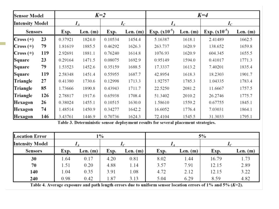
Experimental Results (4/4) Deterministic sensor placement Higher exposure than the randomly generated network topology
 Deterministic sensor placement Higher exposure than the randomly generated network topology")
22
Conclusion This paper introduced the exposure-based model to provide valuable information about the worst case coverage. This paper presented an grid-based approach to identify a minimal exposure path for a given distribution of sensor networks. The proposed Algorithm consists of three parts: 1. Use grid-based approach 2. Apply graph-theoretic abstraction 3. Use Djikstra’s Single-Source-Shortest-Path algorithm

Similar presentations


![Coverage Algorithms Mani Srivastava & Miodrag Potkonjak, UCLA [Project: Sensorware (RSC)] & Mark Jones, Virginia Tech [Project: Dynamic Sensor Nets (ISI-East)]](/15/4573112/big_thumb.jpg "Coverage Algorithms Mani Srivastava & Miodrag Potkonjak, UCLA [Project: Sensorware (RSC)] & Mark Jones, Virginia Tech [Project: Dynamic Sensor Nets (ISI-East)]>")


