Chapter 7 Packet-Switching Networks

Chapter 7 Packet-Switching Networks
Network Services and Internal Network Operation Packet Network Topology Datagrams and Virtual Circuits Routing in Packet Networks Shortest Path Routing ATM Networks Traffic Management

Network Services and Internal Network Operation

Network Layer Network Layer: the most complex layer
Requires the coordinated actions of multiple, geographically distributed network elements (switches & routers) Must be able to deal with very large scales Billions of users (people & communicating devices) Biggest Challenges Addressing: where should information be directed to? Routing: what path should be used to get information there?

Packet Switching Transfer of information as payload in data packets
Network Transfer of information as payload in data packets Packets undergo random delays & possible loss Different applications impose differing requirements on the transfer of information

Network Service End system β Physical layer Data link α Network Transport Messages Segments service Network layer can offer a variety of services to transport layer Connection-oriented service or connectionless service Best-effort or delay/loss guarantees

Network Service vs. Operation
Connectionless Datagram Transfer Connection-Oriented Reliable and possibly constant bit rate transfer Internal Network Operation Connectionless IP Connection-Oriented Telephone connection ATM Various combinations are possible Connection-oriented service over Connectionless operation Connectionless service over Connection-Oriented operation Context & requirements determine what makes sense

Complexity at the Edge or in the Core?
1 3 2 Medium A B C 4 End system α β Network Physical layer entity Data link layer entity Network layer entity Transport layer entity

The End-to-End Argument for System Design
An end-to-end function is best implemented at a higher level than at a lower level End-to-end service requires all intermediate components to work properly Higher-level better positioned to ensure correct operation Example: stream transfer service Establishing an explicit connection for each stream across network requires all network elements (NEs) to be aware of connection; All NEs have to be involved in re-establishment of connections in case of network fault In connectionless network operation, NEs do not deal with each explicit connection and hence are much simpler in design

Network Layer Functions
Essential Routing: mechanisms for determining the set of best paths for routing packets requires the collaboration of network elements Forwarding: transfer of packets from NE inputs to outputs Priority & Scheduling: determining order of packet transmission in each NE Optional: congestion control, segmentation & reassembly, security

Packet Network Topology

End-to-End Packet Network
Packet networks very different than telephone networks Individual packet streams are highly bursty Statistical multiplexing is used to concentrate streams User demand can undergo dramatic change Peer-to-peer applications stimulated huge growth in traffic volumes Internet structure highly decentralized Paths traversed by packets can go through many networks controlled by different organizations No single entity responsible for end-to-end service

Access Multiplexing Access MUX To packet network Packet traffic from users multiplexed at access to network into aggregated streams DSL traffic multiplexed at DSL Access Mux Cable modem traffic multiplexed at Cable Modem Termination System

Oversubscription Access Multiplexer
N subscribers c bps to mux Each subscriber active r/c of time Mux has C=nc bps to network Oversubscription rate: N/n Find n so that at most 1% overflow probability Feasible oversubscription rate increases with size • • • Nr Nc r nc N r/c n N/n 10 0.01 1 10 extremely lightly loaded users 0.05 3 3.3 10 very lightly loaded user 0.1 4 2.5 10 lightly loaded users 20 6 20 lightly loaded users 40 9 4.4 40 lightly loaded users 100 18 5.5 100 lightly loaded users

Home LANs Home Router LAN Access using Ethernet or WiFi (IEEE 802.11)
packet network Home Router LAN Access using Ethernet or WiFi (IEEE ) Private IP addresses in Home ( x) using Network Address Translation (NAT) Single global IP address from ISP issued using Dynamic Host Configuration Protocol (DHCP)

LAN Concentration Switch / Router             LAN Hubs and switches in the access network also aggregate packet streams that flows into switches and routers

To Internet or wide area network
Campus Network Servers have redundant connectivity to backbone Organization Servers To Internet or wide area network s s Gateway Backbone R R R S S S Departmental Server R R R s s High-speed campus backbone net connects dept routers s Only outgoing packets leave LAN through router s s s s s s

Connecting to Internet Service Provider
Border routers Campus Network Border routers Interdomain level Autonomous system or domain Intradomain level s LAN network administered by single organization s s

Internet Backbone National Service Provider A National Service Provider B National Service Provider C NAP Private peering Network Access Points: set up during original commercialization of Internet to facilitate exchange of traffic Private Peering Points: two-party inter-ISP agreements to exchange traffic

NAP (a) (b) RA Route RB Server LAN RC National Service Provider A
National Service Provider B National Service Provider C LAN (a) (b) Private peering

Key Role of Routing How to get packet from here to there?
Decentralized nature of Internet makes routing a major challenge Interior gateway protocols (IGPs) are used to determine routes within a domain Exterior gateway protocols (EGPs) are used to determine routes across domains Routes must be consistent & produce stable flows Scalability required to accommodate growth Hierarchical structure of IP addresses essential to keeping size of routing tables manageable

Datagrams and Virtual Circuits

The Switching Function
Dynamic interconnection of inputs to outputs Enables dynamic sharing of transmission resource Two fundamental approaches: Connectionless Connection-Oriented: Call setup control, Connection control Backbone Network Access Network Switch

Packet Switching Network
Transfers packets between users Transmission lines + packet switches (routers) Origin in message switching Two modes of operation: Connectionless Virtual Circuit Packet switch Network Transmission line User 7-9 The text boxes are callouts or labels.

Message Switching Message switching invented for telegraphy
Entire messages multiplexed onto shared lines, stored & forwarded Headers for source & destination addresses Routing at message switches Connectionless Switches Message Destination Source

Message Switching Delay
Source Destination T  Minimum delay = 3 + 3T Switch 1 Switch 2 Additional queueing delays possible at each link

Long Messages vs. Packets
1 Mbit message source dest BER=p=10-6 BER=10-6 How many bits need to be transmitted to deliver message? Approach 1: send 1 Mbit message Probability message arrives correctly On average it takes about 3 transmissions/hop Total # bits transmitted ≈ 6 Mbits Approach 2: send kbit packets Probability packet arrives correctly On average it takes about 1.1 transmissions/hop Total # bits transmitted ≈ 2.2 Mbits

Packet Switching - Datagram
Messages broken into smaller units (packets) Source & destination addresses in packet header Connectionless, packets routed independently (datagram) Packet may arrive out of order Pipelining of packets across network can reduce delay, increase throughput Lower delay than message switching, suitable for interactive traffic Packet 2 Packet 1

Packet Switching Delay
Assume three packets corresponding to one message traverse same path t Delay 3 1 2 Minimum Delay = 3τ + 5(T/3) (single path assumed) Additional queueing delays possible at each link Packet pipelining enables message to arrive sooner

Delay for k-Packet Message over L Hops
3 1 2 3 + 2(T/3) first bit received 3 + 3(T/3) first bit released 3 + 5 (T/3) last bit released L + (L-1)P first bit received L + LP first bit released L + LP + (k-1)P last bit released where T = k P 3 hops L hops Source Destination Switch 1 Switch 2 

Routing Tables in Datagram Networks
Destination address Output port 1345 12 2458 7 0785 6 1566 Route determined by table lookup Routing decision involves finding next hop in route to given destination Routing table has an entry for each destination specifying output port that leads to next hop Size of table becomes impractical for very large number of destinations

Example: Internet Routing
Internet protocol uses datagram packet switching across networks Networks are treated as data links Hosts have two-port IP address: Network address + Host address Routers do table lookup on network address This reduces size of routing table In addition, network addresses are assigned so that they can also be aggregated Discussed as CIDR in Chapter 8

Packet Switching – Virtual Circuit
Call set-up phase sets ups pointers in fixed path along network All packets for a connection follow the same path Abbreviated header identifies connection on each link Packets queue for transmission Variable bit rates possible, negotiated during call set-up Delays variable, cannot be less than circuit switching

Connection Setup Signaling messages propagate as route is selected
SW 1 SW 2 SW n Connect request Connect confirm … Signaling messages propagate as route is selected Signaling messages identify connection and setup tables in switches Typically a connection is identified by a local tag, Virtual Circuit Identifier (VCI) Each switch only needs to know how to relate an incoming tag in one input to an outgoing tag in the corresponding output Once tables are setup, packets can flow along path

Connection Setup Delay
3 1 2 Release Connect request CR Connect confirm CC Connection setup delay is incurred before any packet can be transferred Delay is acceptable for sustained transfer of large number of packets This delay may be unacceptably high if only a few packets are being transferred

Virtual Circuit Forwarding Tables
Each input port of packet switch has a forwarding table Lookup entry for VCI of incoming packet Determine output port (next hop) and insert VCI for next link Very high speeds are possible Table can also include priority or other information about how packet should be treated Input VCI Output port 15 58 13 7 27 12 44 23 16 34

Cut-Through switching
3 1 2 Minimum delay = 3 + T t Source Destination Switch 1 Switch 2 Some networks perform error checking on header only, so packet can be forwarded as soon as header is received & processed Delays reduced further with cut-through switching

Message vs. Packet Minimum Delay
L t + L T = L t + (L – 1) T + T Packet L t + L P + (k – 1) P = L t + (L – 1) P + T Cut-Through Packet (Immediate forwarding after header) = L t + T Above neglect header processing delays

Example: ATM Networks All information mapped into short fixed-length packets called cells Connections set up across network Virtual circuits established across networks Tables setup at ATM switches Several types of network services offered Constant bit rate connections Variable bit rate connections

Datagrams and Virtual Circuits Structure of a Packet Switch

Packet Switch: Intersection where Traffic Flows Meet
• • • • • • 1 1 2 2   N N Inputs contain multiplexed flows from access muxs & other packet switches Flows demultiplexed at input, routed and/or forwarded to output ports Packets buffered, prioritized, and multiplexed on output lines

Generic Packet Switch “Unfolded” View of Switch Ingress Line Cards
Header processing Demultiplexing Routing in large switches Controller Routing in small switches Signalling & resource allocation Interconnection Fabric Transfer packets between line cards Egress Line Cards Scheduling & priority Multiplexing Controller 1 2 3 N Line card Interconnection fabric Input ports Output ports Data path Control path (a) …

Line Cards Folded View 1 circuit board is ingress/egress line card
Interconnection fabric Transceiver Framer Network processor Backplane transceivers To physical ports switch other line cards Folded View 1 circuit board is ingress/egress line card Physical layer processing Data link layer processing Network header processing Physical layer across fabric + framing

Shared Memory Packet Switch
Ingress Processing Output Buffering Connection Control 1 1 Queue Control 2 2 3 3 Shared Memory … … N N Small switches can be built by reading/writing into shared memory

Crossbar Switches … … … …
(a) Input buffering (b) Output buffering Inputs Inputs 1 3 1 2 8 3 2 3 3 … … N N … … 1 2 3 N 1 2 3 N Outputs Outputs Large switches built from crossbar & multistage space switches Requires centralized controller/scheduler (who sends to whom when) Can buffer at input, output, or both (performance vs complexity)

Self-Routing Switches
1 2 Inputs Outputs 3 4 5 6 7 Stage 1 Stage 2 Stage 3 Self-routing switches do not require controller Output port number determines route 101 → (1) lower port, (2) upper port, (3) lower port

Routing in Packet Networks

Routing in Packet Networks
1 2 3 4 5 6 Node (switch or router) Three possible (loopfree) routes from 1 to 6: 1-3-6, , Which is “best”? Min delay? Min hop? Max bandwidth? Min cost? Max reliability?

Creating the Routing Tables
Need information on state of links Link up/down; congested; delay or other metrics Need to distribute link state information using a routing protocol What information is exchanged? How often? Exchange with neighbors; Broadcast or flood Need to compute routes based on information Single metric; multiple metrics Single route; alternate routes

Routing Algorithm Requirements
Responsiveness to changes Topology or bandwidth changes, congestion Rapid convergence of routers to consistent set of routes Freedom from persistent loops Optimality Resource utilization, path length Robustness Continues working under high load, congestion, faults, equipment failures, incorrect implementations Simplicity Efficient software implementation, reasonable processing load

Centralized vs Distributed Routing
Centralized Routing All routes determined by a central node All state information sent to central node Problems adapting to frequent topology changes Does not scale Distributed Routing Routes determined by routers using distributed algorithm State information exchanged by routers Adapts to topology and other changes Better scalability

Static vs Dynamic Routing
Static Routing Set up manually, do not change; requires administration Works when traffic predictable & network is simple Used to override some routes set by dynamic algorithm Used to provide default router Dynamic Routing Adapt to changes in network conditions Automated Calculates routes based on received updated network state information

Routing in Virtual-Circuit Packet Networks
1 2 3 4 5 6 A B C D 7 8 Switch or router Host VCI Route determined during connection setup Tables in switches implement forwarding that realizes selected route

Routing Tables in VC Packet Networks
Incoming Outgoing Node VCI Node VCI A A A A B B B B C C D D Node 1 Node 2 Node 3 Node 4 Node 6 Node 5 Example: VCI from A to D From A & VCI 5 → 3 & VCI 3 → 4 & VCI 4 → 5 & VCI 5 → D & VCI 2

Routing Tables in Datagram Packet Networks
Node 1 Node 2 Node 3 Node 4 Node 6 Node 5 Destination Next node

Non-Hierarchical Addresses and Routing
R1 1 2 5 4 3 … … … … R2 No relationship between addresses & routing proximity Routing tables require 16 entries each

Hierarchical Addresses and Routing
R1 R2 1 2 5 4 3 Prefix indicates network where host is attached Routing tables require 4 entries each

Flat vs Hierarchical Routing
Flat Routing All routers are peers Does not scale Hierarchical Routing Partitioning: Domains, autonomous systems, areas... Some routers part of routing backbone Some routers only communicate within an area Efficient because it matches typical traffic flow patterns Scales

Specialized Routing Flooding Deflection Routing
Useful in starting up network Useful in propagating information to all nodes Deflection Routing Fixed, preset routing procedure No route synthesis

Flooding Send a packet to all nodes in a network
No routing tables available Need to broadcast packet to all nodes (e.g. to propagate link state information) Approach Send packet on all ports except one where it arrived Exponential growth in packet transmissions

1 2 3 4 5 6 Flooding is initiated from Node 1: Hop 1 transmissions

Limited Flooding Time-to-Live field in each packet limits number of hops to certain diameter Each switch adds its ID before flooding; discards repeats Source puts sequence number in each packet; switches records source address and sequence number and discards repeats

Deflection Routing Network nodes forward packets to preferred port
If preferred port busy, deflect packet to another port Works well with regular topologies Manhattan street network Rectangular array of nodes Nodes designated (i,j) Rows alternate as one-way streets Columns alternate as one-way avenues Bufferless operation is possible Proposed for optical packet networks All-optical buffering currently not viable

Tunnel from last column to first column or vice versa
0,0 0,1 0,2 0,3 1,0 1,1 1,2 1,3 2,0 2,1 2,2 2,3 3,0 3,1 3,2 3,3 Tunnel from last column to first column or vice versa

Example: Node (0,2)→(1,0) busy 0,0 0,1 0,2 0,3 1,0 1,1 1,2 1,3 2,0 2,1
2,2 2,3 3,0 3,1 3,2 3,3

Shortest Path Routing

Shortest Paths & Routing
Many possible paths connect any given source and to any given destination Routing involves the selection of the path to be used to accomplish a given transfer Typically it is possible to attach a cost or distance to a link connecting two nodes Routing can then be posed as a shortest path problem

Routing Metrics Means for measuring desirability of a path
Path Length = sum of costs or distances Possible metrics Hop count: rough measure of resources used Reliability: link availability; BER Delay: sum of delays along path; complex & dynamic Bandwidth: “available capacity” in a path Load: Link & router utilization along path Cost: $$$

Shortest Path Approaches
Distance Vector Protocols Neighbors exchange list of distances to destinations Best next-hop determined for each destination Ford-Fulkerson (distributed) shortest path algorithm Link State Protocols Link state information flooded to all routers Routers have complete topology information Shortest path (& hence next hop) calculated Dijkstra (centralized) shortest path algorithm

Distance Vector Do you know the way to San Jose?

Distance Vector Local Signpost Table Synthesis Direction
Routing Table For each destination list: Next Node Table Synthesis Neighbors exchange table entries Determine current best next hop Inform neighbors Periodically After changes dest next dist

Shortest Path to SJ San Jose j i Dj Di
Focus on how nodes find their shortest path to a given destination node, i.e. SJ San Jose Dj Cij j i Di If Di is the shortest distance to SJ from i and if j is a neighbor on the shortest path, then Di = Cij + Dj

But we don’t know the shortest paths
i only has local info from neighbors San Jose Dj' j' Cij' Dj j Cij i Pick current shortest path Cij” Di j" Dj"

Why Distance Vector Works
SJ sends accurate info San Jose Accurate info about SJ ripples across network, Shortest Path Converges 1 Hop From SJ 2 Hops From SJ 3 Hops From SJ Hop-1 nodes calculate current (next hop, dist), & send to neighbors

Bellman-Ford Algorithm
Consider computations for one destination d Initialization Each node table has 1 row for destination d Distance of node d to itself is zero: Dd=0 Distance of other node j to d is infinite: Dj=, for j d Next hop node nj = -1 to indicate not yet defined for j  d Send Step Send new distance vector to immediate neighbors across local link Receive Step At node i, find the next hop that gives the minimum distance to d, Minj { Cij + Dj } Replace old (nj, Dj(d)) by new (nj*, Dj*(d)) if new next node or distance Go to send step

Bellman-Ford Algorithm
Now consider parallel computations for all destinations d Initialization Each node has 1 row for each destination d Distance of node d to itself is zero: Dd(d)=0 Distance of other node j to d is infinite: Dj(d)=  , for j  d Next node nj = -1 since not yet defined Send Step Send new distance vector to immediate neighbors across local link Receive Step For each destination d, find the next hop that gives the minimum distance to d, Minj { Cij+ Dj(d) } Replace old (nj, Di(d)) by new (nj*, Dj*(d)) if new next node or distance found Go to send step

San Jose Initial (-1, ) 1 2 3 Table entry @ node 3 for dest SJ
Iteration Node 1 Node 2 Node 3 Node 4 Node 5 Initial (-1, ) 1 2 3 Table entry @ node 3 for dest SJ Table entry @ node 1 for dest SJ 3 1 5 4 6 2 San Jose

San Jose Initial (-1, ) 1 (6,1) (6,2) 2 3 1 2 D3=D6+1 n3=6 D6=0 3 1 5
Iteration Node 1 Node 2 Node 3 Node 4 Node 5 Initial (-1, ) 1 (6,1) (6,2) 2 3 D3=D6+1 n3=6 D6=0 1 3 1 5 4 6 2 San Jose 2 D6=0 D5=D6+2 n5=6

San Jose Initial (-1, ) 1 (6, 1) (6,2) 2 (3,3) (5,6) 3 3 1 3 6 2 3 1
Iteration Node 1 Node 2 Node 3 Node 4 Node 5 Initial (-1, ) 1 (6, 1) (6,2) 2 (3,3) (5,6) 3 3 1 3 1 5 4 6 2 3 San Jose 6 2

San Jose Initial (-1, ) 1 (6, 1) (6,2) 2 (3,3) (5,6) 3 (4,4) 1 3 3 6
Iteration Node 1 Node 2 Node 3 Node 4 Node 5 Initial (-1, ) 1 (6, 1) (6,2) 2 (3,3) (5,6) 3 (4,4) 1 3 3 1 5 4 6 2 3 San Jose 6 4 2

Network disconnected; Loop created between nodes 3 and 4
Iteration Node 1 Node 2 Node 3 Node 4 Node 5 Initial (3,3) (4,4) (6, 1) (6,2) 1 (4, 5) 2 3 1 5 3 3 1 5 4 6 2 3 San Jose 4 2 Network disconnected; Loop created between nodes 3 and 4

Node 4 could have chosen 2 as next node because of tie
Iteration Node 1 Node 2 Node 3 Node 4 Node 5 Initial (3,3) (4,4) (6, 1) (6,2) 1 (4, 5) 2 (3,7) (5,5) 3 5 7 3 3 1 5 4 6 2 5 3 San Jose 2 4 Node 4 could have chosen 2 as next node because of tie

San Jose Initial (3,3) (4,4) (6, 1) (6,2) 1 (4, 5) 2 (3,7) (5,5) 3
Iteration Node 1 Node 2 Node 3 Node 4 Node 5 Initial (3,3) (4,4) (6, 1) (6,2) 1 (4, 5) 2 (3,7) (5,5) 3 (4,6) (4, 7) 5 7 7 3 1 5 4 6 2 5 San Jose 2 4 6 Node 2 could have chosen 5 as next node because of tie

San Jose 1 (3,3) (4,4) (4, 5) (6,2) 2 (3,7) (2,5) 3 (4,6) (4, 7) (5,5)
Iteration Node 1 Node 2 Node 3 Node 4 Node 5 1 (3,3) (4,4) (4, 5) (6,2) 2 (3,7) (2,5) 3 (4,6) (4, 7) (5,5) 4 (2,9) 7 7 9 3 5 4 6 2 1 5 San Jose 6 2 Node 1 could have chose 3 as next node because of tie

Counting to Infinity Problem
3 1 2 4 X (a) (b) Nodes believe best path is through each other (Destination is node 4) Update Node 1 Node 2 Node 3 Before break (2,3) (3,2) (4, 1) After break 1 (3,4) 2 (2,5) 3 (3,6) 4 (2,7) 5 (3,8) …

Problem: Bad News Travels Slowly
Remedies Split Horizon Do not report route to a destination to the neighbor from which route was learned Poisoned Reverse Report route to a destination to the neighbor from which route was learned, but with infinite distance Breaks erroneous direct loops immediately Does not work on some indirect loops

Split Horizon with Poison Reverse
3 1 2 4 X (a) (b) Nodes believe best path is through each other Update Node 1 Node 2 Node 3 Before break (2, 3) (3, 2) (4, 1) After break (-1, ) Node 2 advertizes its route to 4 to node 3 as having distance infinity; node 3 finds there is no route to 4 1 Node 1 advertizes its route to 4 to node 2 as having distance infinity; node 2 finds there is no route to 4 2 Node 1 finds there is no route to 4

Link-State Algorithm ID’s of its neighbors: Ni=set of neighbors of i
Basic idea: two step procedure Each source node gets a map of all nodes and link metrics (link state) of the entire network Find the shortest path on the map from the source node to all destination nodes Broadcast of link-state information Every node i in the network broadcasts to every other node in the network: ID’s of its neighbors: Ni=set of neighbors of i Distances to its neighbors: {Cij | j Ni} Flooding is a popular method of broadcasting packets

Dijkstra Algorithm: Finding shortest paths in order
Find shortest paths from source s to all other destinations Closest node to s is 1 hop away 2nd closest node to s is 1 hop away from s or w” 3rd closest node to s is 1 hop away from s, w”, or x w' w' z w x x s z' w" w" x'

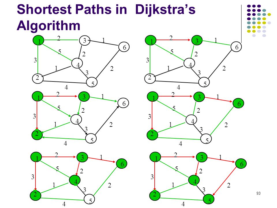
Dijkstra’s algorithm N: set of nodes for which shortest path already found Initialization: (Start with source node s) N = {s}, Ds = 0, “s is distance zero from itself” Dj=Csj for all j  s, distances of directly-connected neighbors Step A: (Find next closest node i) Find i  N such that Di = min Dj for j  N Add i to N If N contains all the nodes, stop Step B: (update minimum costs) For each node j  N Dj = min (Dj, Di+Cij) Go to Step A Minimum distance from s to j through node i in N

Execution of Dijkstra’s algorithm
 1 2 4 5 6 3 3 1 2 4 5 6 1 2 4 5 6 3 1 2 4 5 6 3 1 2 4 5 6 3 1 2 4 5 6 3 1 2 4 5 6 3    Iteration N D2 D3 D4 D5 D6 Initial {1} 3 2 5  1 {1,3} 4 {1,2,3} 7 {1,2,3,6} {1,2,3,4,6} {1,2,3,4,5,6}     

Shortest Paths in Dijkstra’s Algorithm
1 2 4 5 6 3 3 1 2 4 5 6 1 2 4 5 6 3 1 2 4 5 6 3 1 2 4 5 6 3 1 2 4 5 6 3

Reaction to Failure If a link fails,
Router sets link distance to infinity & floods the network with an update packet All routers immediately update their link database & recalculate their shortest paths Recovery very quick But watch out for old update messages Add time stamp or sequence # to each update message Check whether each received update message is new If new, add it to database and broadcast If older, send update message on arriving link

Why is Link State Better?
Fast, loopless convergence Support for precise metrics, and multiple metrics if necessary (throughput, delay, cost, reliability) Support for multiple paths to a destination algorithm can be modified to find best two paths

Source Routing Source host selects path that is to be followed by a packet Strict: sequence of nodes in path inserted into header Loose: subsequence of nodes in path specified Intermediate switches read next-hop address and remove address Source host needs link state information or access to a route server Source routing allows the host to control the paths that its information traverses in the network Potentially the means for customers to select what service providers they use

Example 3,6,B 6,B 1,3,6,B 1 3 B 6 A 4 B Source host 2 Destination host
5

ATM Networks

Asynchronous Tranfer Mode (ATM)
Packet multiplexing and switching Fixed-length packets: “cells” Connection-oriented Rich Quality of Service support Conceived as end-to-end Supporting wide range of services Real time voice and video Circuit emulation for digital transport Data traffic with bandwidth guarantees Detailed discussion in Chapter 9

ATM Networking ATM Network
Voice Video Packet Voice Video Packet ATM Adaptation Layer ATM Adaptation Layer ATM Network End-to-end information transport using cells 53-byte cell provide low delay and fine multiplexing granularity Support for many services through ATM Adaptation Layer

TDM vs. Packet Multiplexing
Variable bit rate Delay Burst traffic Processing TDM Multirate only Low, fixed Inefficient Minimal, very high speed Packet Easily handled Variable Efficient Header & packet processing required    * *In mid-1980s, packet processing mainly in software and hence slow; By late 1990s, very high speed packet processing possible

ATM: Attributes of TDM & Packet Switching
MUX Wasted bandwidth ATM TDM Voice Data packets Images 1 2 3 4 Packet structure gives flexibility & efficiency Synchronous slot transmission gives high speed & density Packet Header

ATM Switching Switch carries out table translation and routing Switch
2 3 N 1 Switch 5 6 video voice data 25 32 61 75 67 39 … ATM switches can be implemented using shared memory, shared backplanes, or self-routing multi-stage fabrics

ATM Virtual Connections
Virtual connections setup across network Connections identified by locally-defined tags ATM Header contains virtual connection information: 8-bit Virtual Path Identifier 16-bit Virtual Channel Identifier Powerful traffic grooming capabilities Multiple VCs can be bundled within a VP Similar to tributaries with SONET, except variable bit rates possible Virtual paths Physical link Virtual channels

VPI/VCI switching & multiplexing
ATM Sw 1 4 2 3 crossconnect a b c d e VPI 3 VPI 5 VPI 2 VPI 1 Sw = switch Connections a,b,c bundled into VP at switch 1 Crossconnect switches VP without looking at VCIs VP unbundled at switch 2; VC switching thereafter VPI/VCI structure allows creation virtual networks

MPLS & ATM ATM initially touted as more scalable than packet switching
ATM envisioned speeds of Mbps Advances in optical transmission proved ATM to be the less scalable: @ 10 Gbps Segmentation & reassembly of messages & streams into 48-byte cell payloads difficult & inefficient Header must be processed every 53 bytes vs. 500 bytes on average for packets Delay due to 1250 byte packet at 10 Gbps = 1 msec; delay due to 53 byte 150 Mbps ≈ 3 msec MPLS (Chapter 10) uses tags to transfer packets across virtual circuits in Internet

Traffic Management Packet Level Flow Level Flow-Aggregate Level

Traffic Management Vehicular traffic management
Traffic lights & signals control flow of traffic in city street system Objective is to maximize flow with tolerable delays Priority Services Police sirens Cavalcade for dignitaries Bus & High-usage lanes Trucks allowed only at night Packet traffic management Multiplexing & access mechanisms to control flow of packet traffic Objective is make efficient use of network resources & deliver QoS Priority Fault-recovery packets Real-time traffic Enterprise (high-revenue) traffic High bandwidth traffic

Time Scales & Granularities
Packet Level Queueing & scheduling at multiplexing points Determines relative performance offered to packets over a short time scale (microseconds) Flow Level Management of traffic flows & resource allocation to ensure delivery of QoS (milliseconds to seconds) Matching traffic flows to resources available; congestion control Flow-Aggregate Level Routing of aggregate traffic flows across the network for efficient utilization of resources and meeting of service levels “Traffic Engineering”, at scale of minutes to days

End-to-End QoS 1 2 N N – 1 Packet buffer … A packet traversing network encounters delay and possible loss at various multiplexing points End-to-end performance is accumulation of per-hop performances

Scheduling & QoS End-to-End QoS & Resource Control Scheduling Concepts
Buffer & bandwidth control → Performance Admission control to regulate traffic level Scheduling Concepts fairness/isolation priority, aggregation, Fair Queueing & Variations WFQ, PGPS Guaranteed Service WFQ, Rate-control Packet Dropping aggregation, drop priorities

FIFO Queueing All packet flows share the same buffer
Packet buffer Transmission link Arriving packets Packet discard when full All packet flows share the same buffer Transmission Discipline: First-In, First-Out Buffering Discipline: Discard arriving packets if buffer is full (Alternative: random discard; pushout head-of-line, i.e. oldest, packet)

FIFO Queueing Cannot provide differential QoS to different packet flows Different packet flows interact strongly Statistical delay guarantees via load control Restrict number of flows allowed (connection admission control) Difficult to determine performance delivered Finite buffer determines a maximum possible delay Buffer size determines loss probability But depends on arrival & packet length statistics Variation: packet enqueueing based on queue thresholds some packet flows encounter blocking before others higher loss, lower delay

FIFO Queueing with Discard Priority
Packet buffer Transmission link Arriving packets Packet discard when full Class 1 discard Class 2 discard when threshold exceeded (a) (b)

HOL Priority Queueing High priority queue serviced until empty
Transmission link Packet discard when full High-priority packets Low-priority When high-priority queue empty High priority queue serviced until empty High priority queue has lower waiting time Buffers can be dimensioned for different loss probabilities Surge in high priority queue can cause low priority queue to saturate

HOL Priority Features Provides differential QoS
Pre-emptive priority: lower classes invisible Non-preemptive priority: lower classes impact higher classes through residual service times High-priority classes can hog all of the bandwidth & starve lower priority classes Need to provide some isolation between classes Delay Per-class loads (Note: Need labeling)

Earliest Due Date Scheduling
Sorted packet buffer Transmission link Arriving packets Packet discard when full Tagging unit Queue in order of “due date” packets requiring low delay get earlier due date packets without delay get indefinite or very long due dates

Fair Queueing / Generalized Processor Sharing
C bits/second Transmission link Packet flow 1 Packet flow 2 Packet flow n Approximated bit-level round robin service … … Each flow has its own logical queue: prevents hogging; allows differential loss probabilities C bits/sec allocated equally among non-empty queues transmission rate = C / n(t), where n(t)=# non-empty queues Idealized system assumes fluid flow from queues Implementation requires approximation: simulate fluid system; sort packets according to completion time in ideal system

Packet-by-packet system: buffer 1 served first at rate 1;
at t=0 Buffer 2 1 t 2 Fluid-flow system: both packets served at rate 1/2 Both packets complete service at t = 2 Packet-by-packet system: buffer 1 served first at rate 1; then buffer 2 served at rate 1. Packet from buffer 2 being served Packet from buffer 1 being served buffer 2 waiting

Packet from buffer 2 served at rate 1
at t=0 Buffer 2 2 1 t 3 Fluid-flow system: both packets served at rate 1/2 Packet from buffer 2 served at rate 1 Packet-by-packet fair queueing: buffer 2 served at rate 1 Packet from buffer 1 served at rate 1 buffer 2 waiting

Packet-by-packet weighted fair queueing:
Buffer 1 at t=0 Fluid-flow system: packet from buffer 1 served at rate 1/4; Packet from buffer 1 served at rate 1 Buffer 2 at t=0 1 Packet from buffer 2 served at rate 3/4 t 1 2 Packet from buffer 1 waiting Packet-by-packet weighted fair queueing: buffer 2 served first at rate 1; then buffer 1 served at rate 1 1 Packet from buffer 1 served at rate 1 Packet from buffer 2 served at rate 1 t 1 2

Packetized GPS/WFQ Compute packet completion time in ideal system
Sorted packet buffer Transmission link Arriving packets Packet discard when full Tagging unit Compute packet completion time in ideal system add tag to packet sort packet in queue according to tag serve according to HOL

Bit-by-Bit Fair Queueing
Assume n flows, n queues 1 round = 1 cycle serving all n queues If each queue gets 1 bit per cycle, then 1 round = # active queues Round number = number of cycles of service that have been completed rounds Current Round # If packet arrives to idle queue: Finishing time = round number + packet size in bits If packet arrives to active queue: Finishing time = finishing time of last packet in queue + packet size

Number of rounds = Number of bit transmission opportunities
Buffer 1 Buffer 2 Buffer n Number of rounds = Number of bit transmission opportunities Rounds Packet of length k bits begins transmission at this time Packet completes rounds later … Differential Service: If a traffic flow is to receive twice as much bandwidth as a regular flow, then its packet completion time would be half

Computing the Finishing Time
F(i,k,t) = finish time of kth packet that arrives at time t to flow i P(i,k,t) = size of kth packet that arrives at time t to flow i R(t) = round number at time t Generalize so R(t) continuous, not discrete rounds R(t) grows at rate inversely proportional to n(t) Fair Queueing: F(i,k,t) = max{F(i,k-1,t), R(t)} + P(i,k,t) Weighted Fair Queueing: F(i,k,t) = max{F(i,k-1,t), R(t)} + P(i,k,t)/wi

WFQ and Packet QoS WFQ and its many variations form the basis for providing QoS in packet networks Very high-speed implementations available, up to 10 Gbps and possibly higher WFQ must be combined with other mechanisms to provide end-to-end QoS (next section)

Buffer Management Packet drop strategy: Which packet to drop when buffers full Fairness: protect behaving sources from misbehaving sources Aggregation: Per-flow buffers protect flows from misbehaving flows Full aggregation provides no protection Aggregation into classes provided intermediate protection Drop priorities: Drop packets from buffer according to priorities Maximizes network utilization & application QoS Examples: layered video, policing at network edge Controlling sources at the edge

Early or Overloaded Drop
Random early detection: drop pkts if short-term avg of queue exceeds threshold pkt drop probability increases linearly with queue length mark offending pkts improves performance of cooperating TCP sources increases loss probability of misbehaving sources

Random Early Detection (RED)
Packets produced by TCP will reduce input rate in response to network congestion Early drop: discard packets before buffers are full Random drop causes some sources to reduce rate before others, causing gradual reduction in aggregate input rate Algorithm: Maintain running average of queue length If Qavg < minthreshold, do nothing If Qavg > maxthreshold, drop packet If in between, drop packet according to probability Flows that send more packets are more likely to have packets dropped

Packet Drop Profile in RED
Average queue length Probability of packet drop 1 minth maxth full

Traffic Management at the Flow Level

Congestion occurs when a surge of traffic overloads network resources
4 8 6 3 2 1 5 7 Congestion Approaches to Congestion Control: Preventive Approaches: Scheduling & Reservations Reactive Approaches: Detect & Throttle/Discard

Ideal effect of congestion control:
Resources used efficiently up to capacity available Offered load Throughput Controlled Uncontrolled

Open-Loop Control Network performance is guaranteed to all traffic flows that have been admitted into the network Initially for connection-oriented networks Key Mechanisms Admission Control Policing Traffic Shaping Traffic Scheduling

Admission Control Flows negotiate contract with network
Specify requirements: Peak, Avg., Min Bit rate Maximum burst size Delay, Loss requirement Network computes resources needed “Effective” bandwidth If flow accepted, network allocates resources to ensure QoS delivered as long as source conforms to contract Time Bits/second Peak rate Average rate Typical bit rate demanded by a variable bit rate information source

Policing Network monitors traffic flows continuously to ensure they meet their traffic contract When a packet violates the contract, network can discard or tag the packet giving it lower priority If congestion occurs, tagged packets are discarded first Leaky Bucket Algorithm is the most commonly used policing mechanism Bucket has specified leak rate for average contracted rate Bucket has specified depth to accommodate variations in arrival rate Arriving packet is conforming if it does not result in overflow

Leaky Bucket algorithm can be used to police arrival rate of a packet stream
water drains at a constant rate leaky bucket water poured irregularly Leak rate corresponds to long-term rate Bucket depth corresponds to maximum allowable burst arrival 1 packet per unit time Assume constant-length packet as in ATM Let X = bucket content at last conforming packet arrival Let ta – last conforming packet arrival time = depletion in bucket

Leaky Bucket Algorithm
Arrival of a packet at time ta X’ = X - (ta - LCT) X’ < 0? X’ > L? X = X’ + I LCT = ta conforming packet X’ = 0 Nonconforming packet X = value of the leaky bucket counter X’ = auxiliary variable LCT = last conformance time Yes No Depletion rate: 1 packet per unit time L+I = Bucket Depth I = increment per arrival, nominal interarrival time Interarrival time Current bucket content Non-empty empty arriving packet would cause overflow conforming packet

Leaky Bucket Example I = 4 L = 6
L+I Bucket content Time Packet arrival Nonconforming * Non-conforming packets not allowed into bucket & hence not included in calculations

Policing Parameters T = 1 / peak rate MBS = maximum burst size
I = nominal interarrival time = 1 / sustainable rate Time MBS T L I

Dual Leaky Bucket Dual leaky bucket to police PCR, SCR, and MBS:
Tagged or dropped Untagged traffic Incoming traffic PCR = peak cell rate CDVT = cell delay variation tolerance SCR = sustainable cell rate MBS = maximum burst size Leaky bucket 1 SCR and MBS Leaky bucket 2 PCR and CDVT

Traffic Shaping Networks police the incoming traffic flow
Network C Network A Network B Traffic shaping Policing 1 2 3 4 Networks police the incoming traffic flow Traffic shaping is used to ensure that a packet stream conforms to specific parameters Networks can shape their traffic prior to passing it to another network

Leaky Bucket Traffic Shaper
Incoming traffic Shaped traffic Size N Packet Server Buffer incoming packets Play out periodically to conform to parameters Surges in arrivals are buffered & smoothed out Possible packet loss due to buffer overflow Too restrictive, since conforming traffic does not need to be completely smooth

Token Bucket Traffic Shaper
Incoming traffic Shaped traffic Size N Size K Tokens arrive periodically Server Packet Token An incoming packet must have sufficient tokens before admission into the network Token rate regulates transfer of packets If sufficient tokens available, packets enter network without delay K determines how much burstiness allowed into the network

Token Bucket Shaping Effect
The token bucket constrains the traffic from a source to be limited to b + r t bits in an interval of length t b bytes instantly t r bytes/second b + r t

Packet transfer with Delay Guarantees
Bit rate > R > r e.g., using WFQ A(t) = b+rt R(t) No backlog of packets (a) 1 2 Token Shaper bR b R - r (b) Buffer occupancy at 1 Empty t Buffer occupancy at 2 Assume fluid flow for information Token bucket allows burst of b bytes 1 & then r bytes/second Since R>r, buffer 1 never greater than b byte Thus mux < b/R Rate into second mux is r<R, so bytes are never delayed

Delay Bounds with WFQ / PGPS
Assume traffic shaped to parameters b & r schedulers give flow at least rate R>r H hop path m is maximum packet size for the given flow M maximum packet size in the network Rj transmission rate in jth hop Maximum end-to-end delay that can be experienced by a packet from flow i is:

Scheduling for Guaranteed Service
Suppose guaranteed bounds on end-to-end delay across the network are to be provided A call admission control procedure is required to allocate resources & set schedulers Traffic flows from sources must be shaped/regulated so that they do not exceed their allocated resources Strict delay bounds can be met

Current View of Router Function
Classifier Input driver Internet forwarder Pkt. scheduler Output driver Routing Agent Reservation Mgmt. Admission Control [Routing database] [Traffic control database]

Closed-Loop Flow Control
Congestion control feedback information to regulate flow from sources into network Based on buffer content, link utilization, etc. Examples: TCP at transport layer; congestion control at ATM level End-to-end vs. Hop-by-hop Delay in effecting control Implicit vs. Explicit Feedback Source deduces congestion from observed behavior Routers/switches generate messages alerting to congestion

End-to-End vs. Hop-by-Hop Congestion Control
Source Destination Feedback information Packet flow (a) (b)

Traffic Engineering Management exerted at flow aggregate level
Distribution of flows in network to achieve efficient utilization of resources (bandwidth) Shortest path algorithm to route a given flow not enough Does not take into account requirements of a flow, e.g. bandwidth requirement Does not take account interplay between different flows Must take into account aggregate demand from all flows

Shortest path routing congests link 4 to 8
6 3 2 1 5 8 7 (a) (b) Shortest path routing congests link 4 to 8 Better flow allocation distributes flows more uniformly

Chapter 7 Packet-Switching Networks

Similar presentations

Presentation on theme: "Chapter 7 Packet-Switching Networks"— Presentation transcript:

Similar presentations

About project

Feedback

Log in

Auth with social network:

Chapter 7 Packet-Switching Networks

Similar presentations

Presentation on theme: "Chapter 7 Packet-Switching Networks"— Presentation transcript:

Similar presentations

About project

Feedback