1. Manufacturing Systems II
Chris Hicks

2. Topics Group Technology (Cellular Manufacture) Inventory Management
Material Requirements Planning
Just-in-Time Manufacture

3. Cellular Manufacturing

4. References
Apple J.M. (1977) Plant Layout and Material Handling, Wiley, New York.
Askin G.G & Standridge C.R. (1993) Modelling and Analysis of Manufacturing Systems, John Wiley
ISBN
Black J.T. (1991) “The Design of a Factory with a Future”, McGraw-Hill, New York, ISBN

5. References (cont.) Burbidge J.L. (1978)
Principles of Production Control
MacDonald and Evans, England
ISBN
Gallagher C.C. and Knight W.A. (1986)
Group Technology Production Methods in Manufacture
E. Horwood, England ISBN
Hyde W.F. (1981)
Data Analysis for Database Design
Marcel Dekker Inc
ISBN

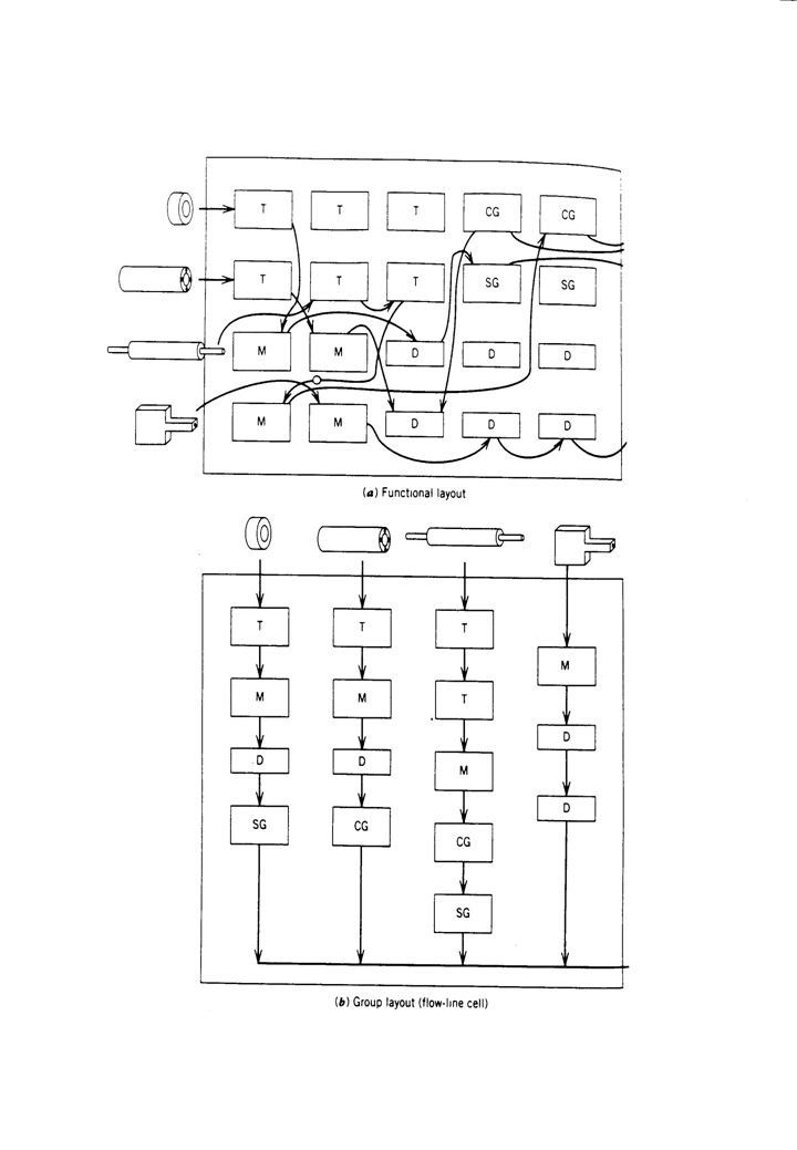
6. Manufacturing Layout
Process (functional) layout, like resources placed together.
Group (cellular) layout, resources to produce like products placed together.

8. Scientific Management
F.W.Taylor 1907
Division of labour - functional specialism
Separation of “doing” and “thinking”
Workers should have exact instructions
Working methods should be standardised
Specialisation led to functional layouts

9. Process Layout Like machines placed together
Labour demarcation / common skills
Robust wrt machine breakdown
Common jigs / fixtures etc.
Sometimes high utilisation
Components travel large distances
High work in progress
Long lead times
Poor throughput efficiency
Often hard to control

10. Group Technology (Cellular Manufacturing)
Group Technology is a manufacturing philosophy with far reaching implications.
The basic concept is to identify and bring together similar parts and processes to take advantage of all the similarities which exist during all stages of design and manufacture.
A cellular manufacturing system is a manufacturing system based upon groups of processes, people and machines to produce a specific family of products with similar manufacturing characteristics (Apple 1977).

11. Cellular Manufacturing
Can be viewed as an attempt to obtain the advantages of flow line systems in previously process based, job shop environments.
First developed in the Soviet Union in 1930s by Mitrofanov.
Early examples referred to as Group Technology.
Promoted by government in 1960s, but very little take up.
In 1978, Burbidge asked “What happened to Group Technology?”
Involves the standardisation of design and process plans.

12. Group (Cellular) Layout
Product focused layout.
Components travel small distances.
Prospect of low work in progress.
Prospect of shorter lead times.
Reduced set-up times.
Design - variety reduction, increased standardisation, easier drawing retrieval.
Control simplified and easier to delegate.
Local storage of tooling.

13. Group (Cellular) Layout
Flexible labour required.
Sometimes lower resource utilisation due to resource duplication.
Organisation should be focused upon the group e.g. planning, control, labour reporting, accounting, performance incentives etc.
Often implemented as a component of JIT with team working, SPC, Quality, TPM etc.
Worker empowerment is important - need people to be dedicated to team success. Cell members should assist decision making.

14. Characteristics of Successful Groups
Characteristic Description
Team Specified team of workers
Products Specified set of products
& no others
Facilities Dedicated machines / equipment
Group layout Dedicated space
Target Common group goal for period
Independence Groups can reach goals
independently
Size Typically 6-15 workers

15. Adapted from Black (1991)

16. Implementation of Cellular Manufacturing
Grouping - identifying which machines to put into each cell.
Cell / layout design - identifying where to put to place machines.
Justification
Human issues

17. Types of Problem
Brown field problem - existing layout, transport, building and infrastructure should be taken into account.
Green field problem - designers are free to select processes, machines, transport, layout, building and infrastructure.
Brown field problems are more constrained, whilst green field problems offer more design choice.

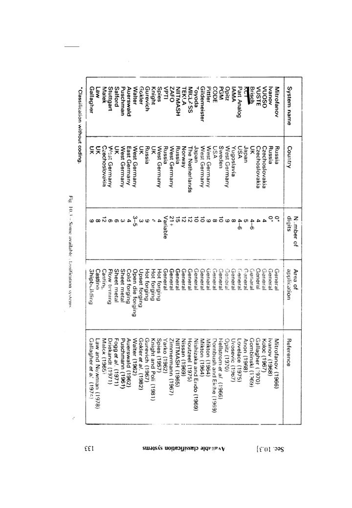
18. Grouping Methods “Eyeballing” Classification of parts
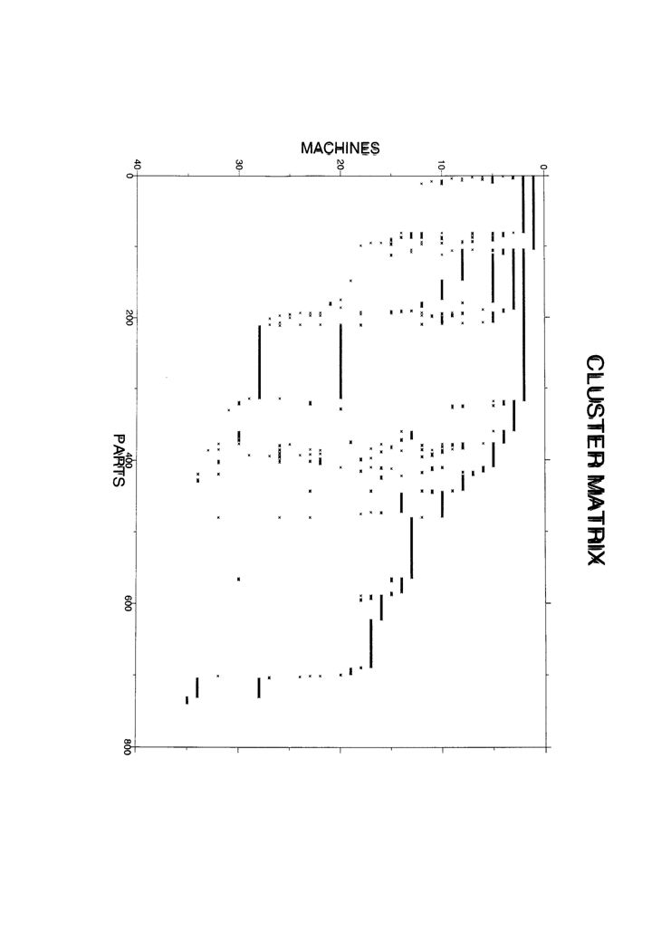
Product Flow Analysis
Cluster Analysis
Matrix methods (e.g. King 1980)
Similarity Coefficient methods
Layout generation without grouping
Beware:
Different methods can give different answers
There may not be clear clusters
Cellular manufacturing not always appropriate

19. Classification of Parts
Based upon coding.
Many schemes available.
Basic idea is to classify according to geometry, similar shapes require similar processes.
Grouping codes together is synonymous with grouping together like parts.
Very prevalent in 1960s and 70s.
Many schemes aimed at particular sectors.

20. Coding issues Part / component population
inclusive should cover all parts.
flexible should deal with future parts / modifications.
should discriminate between parts with different values for key attributes.
Code detail - too much and the code becomes cumbersome - too little and it becomes useless.
Code structure - hierarchical (monocode), chain (polycode) or hybrid.
Digital representation - numeric, alphabetical, combined.

22. Product Flow Analysis Developed by Jack Burbidge (1979).
Uses process routings.
Components with similar routings identified.
Three stages
Factory flow analysis.
Group analysis
Line analysis
(See Askin and Standridge p )

23. Factory Flow Analysis
Link together processes (e.g. machining, welding, pressing) and subprocesses (turning, milling, boring) used by a significant number of parts.
Large departments are formed by combining all related processes.
These are essentially independent plants that manufacture dissimilar products.

24. Group Analysis
Breaks down departments into smaller units that are easier to administer and control.
The objective is to assign machines to groups so as to minimise the amount of material flow between the groups.
Small inexpensive machines are ignored, since they can be replicated if necessary.

25. Group Analysis
Construct a list of parts that require each machine. The machine with fewest part types is the key machine.
A subgroup is formed from all the parts that need this machine plus all the other machines required to make the parts.
A check is then made to see if the subgroup can be subdivided.
If any machine is used by just one part it can be termed “exceptional” and may be removed.

26. Group Analysis
Subgroups with the greatest number of common machine types may be combined to get groups of the desired size.
The combination rule reduces the number of extra machines required and makes it easier to balance machine loads.
Each group must be assigned sufficient machines and staff to produce its assigned parts.

27. Process Plan Example

28. Applying Grouping Steps 1. Identify a key machine. Either E or F.
Create a subgroup to D,E and F.
2. Check for subgroup division. All parts visit F and so subgroup cannot be subdivided. Only part 7 visits machine D so it is exceptional and is removed.
1. Identify an new key machine for remaining 6 parts. A is the new key machine with subgroup A,B,C producing parts 1,2 & 3.
2. Subgroup division - C only used for part 3, therefore exceptional and can be removed.

29. Applying Grouping
1. Identify next key machine. Only parts 4,5, & 6 remain as well as machines C and D.
2. All parts use all machines - no subdivision possible.
3. Cell designer can now recombine the three subgroups into a set of workable groups of desired size.
4. The final solution must provide adequate machine resources in each group for the assigned parts. If exceptional parts exist, or if groups are not self contained, then plans must be made for transport.

30. Rank Order Clustering 1. Evaluate binary value of each row.
2. Swap rows over to get them in rank order.

31. Rank Order Clustering
Next apply same method to the columns

32. Rank Order Clustering
Next swap over columns to get in rank order.

33. Rank Order Clustering ROC has got a solution close to a block
diagonal structure. The process can be
repeated iteratively until a stable solution is
found.

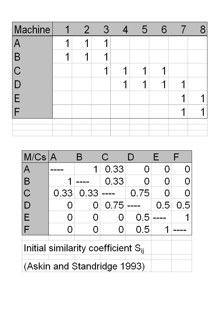
35. Similarity Coefficients
Consider a pair of machines I,j,
ni = number of parts visiting machine i
nj = number of parts visiting machine j
nij = number of parts visiting i and j.
Define similarity coefficient as:
sij = max(nij/ni,nij/nj)
Values near 1 denote high levels of interaction.
Values near 0 denote little or no interaction.

36. Similarity Coefficients

38. Clustering We start with 6 clusters, one for each machine.
With a threshold of T = 1 machines A and B can be grouped. Likewise E and F.
There are several methods for updating similarity coefficients between newly formed clusters and existing clusters.
The single linkage approach uses the maximum Sij for any machine i in the first cluster and any machine j in the second cluster. Therefore any single pair of machines can cause groups to be combined

39. Updating Similarity Coefficients (Using Single Linkage)
Next consider the highest value of T
possible. This gives the cluster CD at
T = 0.75.
The coefficients then need to be updated
again.

40. Dendogram

42. Variety Reduction
Basic principle: always use common designs and components wherever possible.
Modular design.
Standardisation.
Redundant features.
Can base upon geometric series.
Imperial / metric series.
Reduced estimated & work planning.
Simplified stock control.
Less problems with spares.

43. Variety Reduction
May use slightly more expensive parts than necessary.
Increases the volume of production of items.
Reduced planning / jigs and fixtures etc.
Reduced lead times.

44. Product Family Analysis
There are a number of different ways of identifying part families. The following factors should always be considered:
How wide is the range of components?
How static is workload?
What changes are anticipated?
Is Group Technology aimed purely at manufacturing or is standardisation and modularisation of design a major issue?

45. Manufacturing Layout
Concerned with the relative location of major physical manufacturing resources.
A resource may be a machine, department, assembly line etc.
A block plan can be produced that shows the relative positioning of resources.
Evaluation criteria are required such as minimising transport costs, distance travelled etc.

46. Approaches
Many methods are based upon a static deterministic modelling approach.
Dynamic effects may be “guessed” by trying out a variety of scenarios.
Dynamic and stochastic effects may be evaluated by simulation.
A premium may be placed upon favourable attributes
Flexibility dealing with changes in design, demand etc.
Modularity the ability to change the system by adding or removing component parts to meet major changes in demand.
Reliability
Maintainability

47. Line Layout

48. Spine Layout Spine is central core for traffic.
Secondary aisles for traffic into departments
Each department has input /output storage areas along the spine.
Point of use storage reduces material flow.

49. Loop Structure
Circular Structure

50. Layout Configurations
Eli Goldratt I, V, U, W
I layouts have linear flow with no direction changes, empty pallets may go in reverse direction.
V and U lines have more direction changes but may help with empty pallets.
Rectilinear layouts may restrict operators from working multiple machines.
Circular layouts may enable operators to work multiple machines.

51. Analysing Flow
Sting diagrams provide a very quick way to identify the pattern of flow.
Look at performance measures:
Distance travelled per component;
Material handling costs %;
Material handling time %;
Load / unload times;
Number of direction changes;
Number of moves per day;
Many, many more.
Looking at performance measures enables alternative layouts to be evaluated.

52. Measures of Performance
Resource Measures:
Resource utilisation;
Productivity.
Inventory:
work in progress;
queues.
Product:
lead times;
delivery performance;
Quality.
Financial, overhead recovery v.s. ABC costing.

53. Creating Layouts
If there is a dominant flow, such as all parts going from department 1-> 2 -> 3 then the layout should reflect this.
At the other extreme, if the flow between departments is uniformly distributed, then any arrangement may be equally good.
However, most problems will lie between the extremes of dominant and equal flow.

54. Systematic Layout Planning
1. Data collection.
2. Flow analysis.
3 Qualitative considerations.
4. Relationship diagram.
5. Space requirements.
6. Space availability.
7. Space relationship diagram.
8. Modifying considerations and limitations.
9. Evaluation.
(Muther 1973)

55. 1. Data Collection Products to be produced & volumes.
Routing, Bill of Materials, parts lists.
Resources for production, layout & geometrical information.
Timing information - set-up, processing & transfer durations.
Data determines loads & resource utilisation.
Quantity & variety determine appropriate layout type.
A Product-Quantity chart, which is a Pareto analysis of product importance can be used to determine items that justify their own lines or families of parts that justify a cell.

56. Product-Quantity Chart

57. 2. Flow Analysis
Operation process charts determine movement showing major operations, inspections, moves and storage.
Process charts, similar to operation process charts, but more detail.
Flow diagrams.
Flow data can be summarised in From-To charts (like mileage charts in maps)
Volumes
Distance travelled*
Costs*
String diagrams.

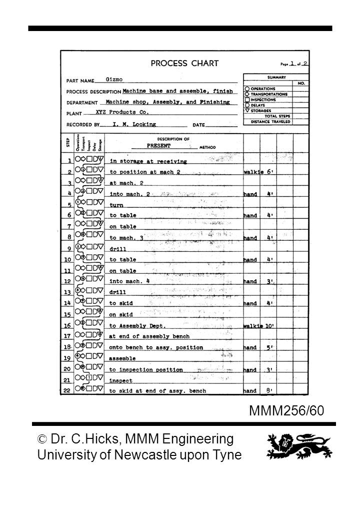
58. Operation Process Chart

59. Process Chart Symbols

61. Flow Diagram
Material flow
Process chart
symbols
Facility layout

62. 3. Qualitative Considerations
REL Chart

63. 4. Relationship Diagram
Combines quantitative and qualitative relationship data.
Provides a mechanism for visualising relationships.

64. 5. Space Requirements
Departmental space requirements need to be estimated.
May have standards that define space requirement for each machine type.
Can work from current space needs.
Can determine space requirement by considering tasks performed, tooling, access, flow of materials etc.

65. 6. Space Availability
Need to accommodate machines, material handling equipment, people, energy transmission, drainage, air lines, communications etc.
If an existing facility is to be used, the available space and constraints need to be accurately defined.
In the case of new facilities there are financial and often planning constraints.Need to consider possibility of future changes in demand or use.

66. 7. Space Relationship Diagram
Represents departments with templates that are proportional in size to space requirements.
Templates can be rearranged to find improved solutions.

67. (a)
(b)
a) Relationship Diagram
b) Space Relationship Diagram

68. 8. Modifying Considerations and Limitations
Steps 1-7 have not taken into account implementation details.
Site specific or operations specific conditions may require adjustments to the layout.
Need to consider:
Utilities, power, heating, light, drainage compressed air etc.
Structural limitations, load-bearing capacity of floors, ceiling heights, columns.
Location of external connections e.g. roads.

69. 9. Evaluation Several alternatives should be considered.
Drawings, flow diagrams etc form the basis of assessment of advantages and disadvantages of each.
Costs / benefits can be attributed to each alternative.
Quality of flow can be evaluated.
Flexibility, maintainability, expandability safety and ease of operations should be reviewed.

70. Computerised Layout Planning
Improvement algorithms are based upon an initial layout. They generate improvements by rearrangement. Suitable for brown field sites. Examples CRAFT (Armour & Buffa 1963)
Construction algorithms start with a blank shop floor and add machines to it. Suitable for green field sites. Example: ALDEP (Seehof & Evans 1967), CORELP (Parsaei et al 1987), SHAPE (Hassan et al 1986).
Hybrid algorithms include both construction and improvement algorithms.

71. Computerised Relative Allocation of Facilities (CRAFT)
Creates layouts by exchanging machine pairs and then evaluating the layout.
When all pairs of exchanges have been completed, the exchange with the best evaluation is chosen and a new layout in generated.
This process is repeated until no improvement can be made through exchanges.

72. Automated Layout Design Program (ALDEP)
A machine is randomly selected and added to the layout.
The closeness of all the remaining machines to it is calculated. The “closest” machine is added. This is repeated until all machines have been placed.
Once a machine has been placed, it is fixed. This makes it difficult to find good solutions.
Often use an improvement algorithm to improve layout produced.

73. Construction Algorithm Differences
Method for election of next machine and its placement.
Evaluation of the relationship between machines already located and the selected machine (e.g. by using different definitions of similarity coefficient).
How the layout is represented.

74. Synthetic Machine Concept
A group of machines form a synthetic machine.
Resource hierarchy flattened.
Framework to assist delegated responsibility.
Local planning, control and work organisation.
Concerned only with cell inputs and outputs.

75. Types of Cell
Highly automated - conveyers, robot handling, Flexible Manufacturing Systems (FMS).
Semi-automated - some automated material handling.
Simple cells without automated material handling.
Work grouped on a single machine using a multi-functional machine tool.
NOTE: Need to find an appropriate mix for given production volumes. Increasing automation normally increases overheads and reduces flexibility.

76. Supporting Techniques
Statistical process control.
Quality Circles.
Team working.
Empowerment.
Visible performance measures.
Total preventative maintenance.
Single minute exchange of dies.
Simple machine concept.

77. Case Study 1 World class automotive components supplier.
Adopted lean manufacturing practices yet productivity still 50% of Japanese sister plant.
WHY?

78. Findings Layout - rectilinear v.s clusters. Supervision of resources.
Smallest machine concept.
Flexible resource variable.
Cost of capital and accounting philosophies.

79. Case Study 2 SME supplier of orthotics (surgical appliances).
Very long delivery.
High work in progress.
How can situation be improved?

80. Solution Business process analysis: Non physical processes;
Target queuing by streamlining processes or increasing capacity.
Result:
Lead time 14 weeks to 4;
Cash flow improved by £300k on £2M turnover.

81. Other Key Issues Batch sizes Set-up Machining Transfer
Effect on other measures of performance.

85. Hints Look at the material flow Try to simplify
Think about removing in-process inventory
Think about the operators
Consider other layout constraints

89. Inventory Management

90. Inventory Money invested in materials 3 Types of inventory
Raw materials
Work in progress
Finished goods

91. Advantages of Inventory
Raw materials offset lead time
Work in progress offsets disturbances in the production system and may help keep resource utilisation high
Finished goods stocks enable fast delivery
Economic order quantity methods claim to claim
People feel busy
Process “decoupling”

92. Inventory: Disadvantages
Expensive to keep
Interest on capital
Storage costs
Adverse effect on cash flow and liquidity
Risk of obsolescence
Lack of flexibility
Masks problems with manufacturing system
Difficult to control

93. Types of Demand Independent
Demand for an item is independent of the demand for another item
Dependant
Demand for an item is linked to the demand for another item
Product structure defines dependencies

94. Inventory Control
“The activities and techniques of maintaining stock items at desired levels, whether they are raw materials, work in progress or finished products”

95. Inventory Control Decisions
How many?
(lot size or order quantity
When
timing or order point

96. Independent Demand
Fixed order quantity (FOQ) systems order a predetermined quantity of items when stock levels drop below a predetermined level e.g. 2 bin system
Economic order quantity systems aim to minimise the combination of ordering and carrying costs. They make a number of assumptions:
annual demand can be estimated
demand is uniform
no quantity discounts
Ignores the costs associated with stock outs

97. Dependent Demand Demand for one item linked to the demand for another
Producing an assembly causes dependent demand for all the components that go into the assembly
Assembling a car requires one windscreen, 5 wheels, one engine etc.
One engine requires one crankshaft, one cylinder head etc.
One cylinder head requires ….

98. Product Structure

99. Product Structure A B c D E F G H

100. Material Requirements Planning
Method for planning dependent demand
Requirement for subassemblies and components based upon requirements for end items and product structure
Takes into account current stocks of each item to calculate net requirements

101. Material Requirements Planning
End Item Requirements
Stocks
MRP
Product
Structure
Net Requirements

102. ABC Classification Break items into 3 groups:
A - the items that represent 75% of value and 20% volume
B - the items that represent 20% value and 30% volume
C - the items that represent 5% value and 50% volume
This approach is based upon
Parieto analysis

103. Just-in-Time

104. Just-in-Time Approach to achieve excellence in manufacturing
Minimise waste: anything that adds cost but not value
Just the correct quantity
at just the right quality
at just the right time
in the right place

105. Push Scheduling
Manufacturing
Systems
Inventory
“PUSH”

106. Kanban
Japanese word for card
One card
Two card

107. One Card Kanban Item + Kanban Stock Area MC1 MC2 Machine 1 operates
at a constant rate
Kanban

108. Two Card Kanban Item Item + Kanban Stock Area MC1 MC2 “P” Kanban
“C” Kanban
“P” Production Kanban
“C” Conveyance Kanban

109. Pull scheduling 5 2 1 4 3
Manufacturing
System
PULL