CS 347Notes 031 CS 347: Distributed Databases and Transaction Processing Notes03: Query Processing Hector Garcia-Molina.

CS 347Notes 031 CS 347: Distributed Databases and Transaction Processing Notes03: Query Processing Hector Garcia-Molina

CS 347Notes 032 Query Processing Decomposition Localization Optimization

CS 347Notes 033 Decomposition Same as in centralized system Normalization Eliminating redundancy Algebraic rewriting

CS 347Notes 034 Normalization Convert from general language to a “standard” form (e.g., Relational Algebra)

CS 347Notes 035 Example Select A,C From R,S Where (R.B=1 and S.D=2) or (R.C>3 and S.D.=2)  (R.B=1 v R.C>3)  S.D.=2 RS Conjunctive normal form  A, C

CS 347Notes 036 Also: Detect invalid expressions E.g.: Select * from R where R.A =3  R does not have “A” attribute

CS 347Notes 037 Eliminate redundancy E.g.: in conditions: (S.A=1)  (S.A>5)  False (S.A<10)  (S.A<5)  S.A<5

CS 347Notes 038 E.g.: Common sub-expressions UU S  cond  cond T S  cond T RRR

CS 347Notes 039 Algebraic rewriting E.g.: Push conditions down  cond3  cond  cond1  cond2 RS R S

CS 347Notes 0310 After decomposition: –One or more algebraic query trees on relations Localization: –Replace relations by corresponding fragments

CS 347Notes 0311 Localization steps (1) Start with query (2) Replace relations by fragments (3) Push  : up (use CS245 rules) ,  : down (4) Simplify – eliminate unnecessary operations

CS 347Notes 0312 Notation for fragment [R: cond] fragment conditions its tuples satisfy

CS 347Notes 0313 Example A (1)  E=3 R

CS 347Notes 0314 (2)  E=3  [R 1 : E < 10] [R 2 : E  10]

CS 347Notes 0315 (3)   E=3 [R 1 : E < 10] [R 2 : E  10]

CS 347Notes 0316 (3)   E=3 [R 1 : E < 10] [R 2 : E  10] ØØ

CS 347Notes 0317 (4)  E=3 [R 1 : E < 10]

CS 347Notes 0318 Rule 1  C1 [R: c2]   C1 [R: c1  c2] [R: False]  Ø A B

CS 347Notes 0319 In example A:  E=3 [R 2 : E  10]   E=3 [R 2 : E=3  E  10]   E=3 [ R 2 : False]  Ø

CS 347Notes 0320 Example B (1)A=common attribute RS A

CS 347Notes 0321 (2)  A [S 1 : A<5] [S 2 : A  5] [R 1 : A 10]

CS 347Notes 0322 (3)  [R 1 :A<5][S 1 :A<5] [R 1 :A<5][S 2 :A  5] [R 2 :5  A  10][S 1 :A<5] [R 2 :5  A  10][S 2 :A  5] [R 3 :A>10][S 1 :A 10][S 2 :A  5] AAAAAA

CS 347Notes 0323 (3)  [R 1 :A<5][S 1 :A<5] [R 1 :A<5][S 2 :A  5] [R 2 :5  A  10][S 1 :A<5] [R 2 :5  A  10][S 2 :A  5] [R 3 :A>10][S 1 :A 10][S 2 :A  5] AAAAAA

CS 347Notes 0324 (4)  [R 1 :A<5][S 1 :A<5] [R 2 :5  A  10][S 2 :A  5] AAA [R 3 :A>10][S 2 :A  5]

CS 347Notes 0325 Rule 2 [R: C 1 ] [S: C 2 ]  [R S: C 1  C 2  R.A = S.A] AA

CS 347Notes 0326  In step 4 of Example B: [R 1 : A<5] [S 2 : A  5]  [R 1 S 2 : R 1.A < 5  S 2.A  5  R 1.A = S 2.A ]  [R 1 S 2 : False]  Ø AAA

CS 347Notes 0327 Localization with derived fragmentation Example C (2) R 1 : R 2: S 1 :K=R.K S 2 :K=R.K A<10 A  10  R.A<10  R.A  10 K

CS 347Notes 0328 (3)  [R 1 ][S 1 ] [R 1 ][S 2 ] [R 2 ][S 1 ] [R 2 ][S 2 ] KKKK

CS 347Notes 0329 (4)  [R 1 :A<10] S 1 :K=R.K [R 2 :A  10] S 2 :K=R.K  R.A<10  R.A  10 KK

CS 347Notes 0330  In step 4 of Example C: [R 1 :A<10] [S 2 :K=R.K  R.A  10]  [R 1 S 2: R 1.A<10  S 2.K=R.K  R.A  10  R 1.K= S 2.K]  [R 1 S 2 :False ] (K is key of R, R 1 )  Ø KKK

CS 347Notes 0331 (4)  [R 1 :A<10] S 1 :K=R.K [R 2 :A  10] S 2 :K=R.K  R.A<10  R.A  10 KK (4) simplified more:  KK R1R1 S1S1 R2R2 S2S2

CS 347Notes 0332 Localization with vertical fragmentation Example D (1)  A R 1 (K, A, B) R R 2 (K, C, D)

CS 347Notes 0333 (2)  A R 1 R 2 (K, A, B) (K, C, D) K

CS 347Notes 0334 (3)  A  K,A R 1 R 2 (K, A, B) (K, C, D) K not really needed

CS 347Notes 0335 (4)  A R 1 (K, A, B)

CS 347Notes 0336 Rule 3 Given vertical fragmentation of R: R i =  Ai (R), Ai  A Then for any B  A:  B (R) =  B [ R i | B  A i  Ø ] i

CS 347Notes 0337 Localization with hybrid fragmentation Example E R 1 =  k<5 [  k,A R] R 2 =  k  5 [  k,A R] R 3 =  k,B R

CS 347Notes 0338 Query:  A  k=3 R

CS 347Notes 0339 Reduced Query:  A  k=3 R 1

CS 347Notes 0340 Summary - Query Processing Decomposition  Localization  Optimization –Overview –Tricks for joins + other operations –Strategies for optimization

CS 347Notes 0341 Optimization Process: Generate query plans Estimate size of intermediate results Estimate cost of plan ($,time,…) P1P1 P2P2 P3P3 PnPn CnCn C3C3 C2C2 C1C1 pick minimum

CS 347Notes 0342 Differences with centralized optimization: New strategies for some operations (semi-join,range-partitioning, sort,…) Many ways to assign and schedule processors

CS 347Notes 0343 Parallel/distributed sort Input:(a) relation R on single site/disk (b) R fragmented/partitioned by sort attribute (c) R fragmented/partitioned by other attribute

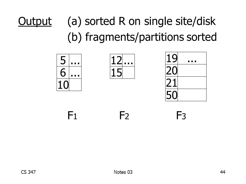
CS 347Notes 0344 Output (a) sorted R on single site/disk (b) fragments/partitions sorted F 1 F 2 F 3 5... 6 10 12... 15 19... 20 21 50

CS 347Notes 0345 Basic sort R(K,…), sort on K Fragmented on K Vector: ko, k 1, … kn 7 3 27 22 11 17 14 1020 k1k1 koko

CS 347Notes 0346 Algorithm: each fragment sorted independently If necessary, ship results

CS 347Notes 0347  Same idea on different architectures: Shared nothing: Shared memory: sorts F1 sorts F2 P1 M P2 M Net F1F1 F2F2 P1P2 M F1F1 F2F2

CS 347Notes 0348 Range partitioning sort R(K,….), sort on K R located at one or more site/disk, not fragmented on K

CS 347Notes 0349 Algorithm: (a) Range partition on K (b) Basic sort Ra Rb R’ 1 R’ 2 R’ 3 ko k1 Local sort R1R1 R2R2 R3R3 Result

CS 347Notes 0350 Selecting a good partition vector RaRbRcRaRbRc 10... 12 4 7... 52 11 14 31... 8 15 11 32 17

CS 347Notes 0351 Example Each site sends to coordinator: –Min sort key –Max sort key –Number of tuples Coordinator computes vector and distributes to sites (also decides # of sites for local sorts)

CS 347Notes 0352 Sample scenario: Coordinator receives: S A : Min=5Max=10# = 10 tuples S B : Min=7Max=17# = 10 tuples

CS 347Notes 0353 Sample scenario: Coordinator receives: S A : Min=5Max=10# = 10 tuples S B : Min=7Max=17# = 10 tuples Expected tuples: 5101520 ko? 2121 [assuming we want to sort at 2 sites]

CS 347Notes 0354 Expected tuples: 5101520 ko? 2121 [assuming we want to sort at 2 sites]

CS 347Notes 0355 Expected tuples=Total tuples with key < ko2 2(ko - 5) + (ko - 7) = 10 3ko = 10 + 10 + 7 = 27 ko = 9 Expected tuples: 5101520 ko? 2121 [assuming we want to sort at 2 sites]

CS 347Notes 0356 Variations Send more info to coordinator –Partition vector for local site Eg. Sa:333 # tuples 5 6 8 10 local vector - Histogram 56789 10

CS 347Notes 0357  More than one round E.g.:(1) Sites send range and # tuples (2) Coordinator returns “preliminary” vector Vo (3) Sites tell coordinator how many tuples in each Vo range (4) Coordinator computes final vector Vf

CS 347Notes 0358  Can you come up with a distributed algorithm? (no coordinator)

CS 347Notes 0359 Parallel external sort-merge Same as range-partition sort, except sort first Ra Rb Local sort Ra’ ko k1 Rb’ Result R1 R2 R3 In order Merge

CS 347Notes 0360 Parallel external sort-merge Same as range-partition sort, except sort first Ra Rb Local sort Ra’ ko k1 Rb’ Result R1 R2 R3 In order Merge Note: can use merging network if available (e.g., Teradata)

CS 347Notes 0361 Parallel/distributed Join Input:Relations R, S May or may not be partitioned Output:R S Result at one or more sites

CS 347Notes 0362 Partitioned Join (Equi-join) Ra S1S1 S2 S3S3 Rb R1R1 R2 R3R3 Sa Sb Sc Local join Result f(A)

CS 347Notes 0363 Notes: Same partition function f is used for both R and S (applied to join attribute) f can be range or hash partitioning Local join can be of any type (use any CS245 optimization) Various scheduling options e.g., (a) partition R; partition S; join (b) partition R; build local hash table for R; partition S and join

CS 347Notes 0364 More notes: We already know why part-join works: R1 R2 R3 S1 S2 S3 R1 S1 R2 S2 R3 S3 Useful to give this type of join a name, because we may want to partition data to make partition-join possible (especially in parallel DB system)    

CS 347Notes 0365 Even more notes: Selecting good partition function f very important: –Number of fragments –Hash function –Partition vector

CS 347Notes 0366 Good partition vector –Goal: | R i |+| S i | the same –Can use coordinator to select

CS 347Notes 0367 Asymmetric fragment + replicate join Ra S S S Rb R1R1 R2R2 R3R3 Sa Sb Local join Result f partition union

CS 347Notes 0368 Notes: Can use any partition function f for R (even round robin) Can do any join — not just equi-join e.g.: R S R.A < S.B

CS 347Notes 0369 General fragment and replicate join f1 partitionn copies of each fragment -> 3 fragments Ra Rb R1 R2 R3 R1 R2 R3

CS 347Notes 0370  S is partitioned in similar fashion Result All nxm pairings of R,S fragments R1S1 R2S1 R3S1 R1S2 R2S2 R3S2

CS 347Notes 0371 Notes: Asymmetric F+R join is special case of general F+R Asymmetric F+R may be good if S small Works for non-equi-joins

CS 347Notes 0372 Semi-join Goal: reduce communication traffic R S  (R S) S or R (S R) or (R S) (S R) AAAAAAAA

CS 347Notes 0373 Example: R S AB A C R S 2a 10 b 25c 30d 3x 10 y 15z 25w 32x

CS 347Notes 0374 Example: R S AB A C R S 2a 10 b 25c 30d 3x 10 y 15z 25w 32x  A R = [2,10,25,30]

CS 347Notes 0375 Example: R S AB A C R S 2a 10 b 25c 30d 3x 10 y 15z 25w 32x  A R = [2,10,25,30] Ans: R S S R = A C 10 y 25 w

CS 347Notes 0376 Computing transmitted data in example: with semi-join R (S R): T = 4 |A| +2 |A+C| + result with join R S: T = 4 |A+B| + result AB A C R S 2a 10 b 25c 30d 3x 10 y 15z 25w 32x

CS 347Notes 0377 Computing transmitted data in example: with semi-join R (S R): T = 4 |A| +2 |A+C| + result with join R S: T = 4 |A+B| + result AB A C R S 2a 10 b 25c 30d 3x 10 y 15z 25w 32x better if say |B| is large

CS 347Notes 0378  In general: Say R is smaller relation (R S) S better than R S if size (  A S) + size (R S) < size (R) AAAA

CS 347Notes 0379 Similar comparisons for other semi-joins Remember: only taking into account transmission cost

CS 347Notes 0380 Trick: Encode  A S (or  A R ) as a bit vector key in S 0 0 1 1 0 1 0 0 0 0 1 0 1 0 0

CS 347Notes 0381  Three way joins with semi-joins Goal: R S T

CS 347Notes 0382  Three way joins with semi-joins Goal: R S T Option 1: R’ S’ T where R’ = R S; S’ = S T

CS 347Notes 0383  Three way joins with semi-joins Goal: R S T Option 1: R’ S’ T where R’ = R S; S’ = S T Option 2: R’’ S’ T where R’’ = R S’; S’ = S T

CS 347Notes 0384  Many options!  Number of semi-join options is exponential in # of relations in join

CS 347Notes 0385 Privacy Preserving Join Site 1 has R(A,B) Site 2 has S(A,C) Want to compute R S Site 1 should NOT discover any S info not in the join Site 2 should NOT discover any R info not in the join R S site 1 site 2

CS 347Notes 0386 Semi-Join Does Not Work If Site 1 sends  A R to Site 2, site 2 leans all keys of R!  A R = (a1, a2, a3, a4) site 1 R A B a1 b1 a2 b2 a3 b3 a4 b4 site 2 S A C a1 c1 a3 c2 a5 c3 a7 c4

CS 347Notes 0387 Fix: Send hashed keys Site 1 hashes each value of A before sending Site 2 hashes (same function) its own A values to see what tuples match  A R = (h(a1), h(a2), h(a3), h(a4)) site 1 R A B a1 b1 a2 b2 a3 b3 a4 b4 site 2 S A C a1 c1 a3 c2 a5 c3 a7 c4 Site 2 sees it has h(a1),h(a3) (a1, c1), (a3, c3)

CS 347Notes 0388 What is problem?  A R = (h(a1), h(a2), h(a3), h(a4)) site 1 R A B a1 b1 a2 b2 a3 b3 a4 b4 site 2 S A C a1 c1 a3 c2 a5 c3 a7 c4 Site 2 sees it has h(a1),h(a3) (a1, c1), (a3, c3)

CS 347Notes 0389 What is problem? Dictionary attack! Site 2 takes all keys, a1, a2, a3... and checks if h(a1), h(a2), h(a3) matches what Site 1 sent...  A R = (h(a1), h(a2), h(a3), h(a4)) site 1 R A B a1 b1 a2 b2 a3 b3 a4 b4 site 2 S A C a1 c1 a3 c2 a5 c3 a7 c4 Site 2 sees it has h(a1),h(a3) (a1, c1), (a3, c3)

CS 347Notes 0390 Adversary Model Honest but Curious –dictionary attack is possible (cheating is internal and can’t be caught) –sending incorrect keys not possible (cheater could be caught)

CS 347Notes 0391 One Solution (Agrawal et al) Use commutative encryption function –E i (x) = x encryption using site i private key –E 1 ( E 2 (x)) = E 2 ( E 1 (X)) –Shorthand for example: E 1 (x) is x E 2 (x) is x E 1 (E 2 (x)) is x

CS 347Notes 0392 Solution: (a1, a2, a3, a4) site 1 R A B a1 b1 a2 b2 a3 b3 a4 b4 site 2 S A C a1 c1 a3 c2 a5 c3 a7 c4 (a1, b1), (a3, b3) (a1, a3, a5, a7) (a1, a2, a3, a4) computes (a1, a3, a5, a7), intersects with (a1, a2, a3, a4)

CS 347Notes 0393 Why does this solution work?

CS 347Notes 0394 Other Privacy Preserving Operations? Inequality join R S Similarity Join R S sim(R.A,S.A)<eR.A > S.A

CS 347Notes 0395 Other parallel operations Duplicate elimination –Sort first (in parallel) then eliminate duplicates in result –Partition tuples (range or hash) and eliminate locally Aggregates –Partition by grouping attributes; compute aggregate locally

CS 347Notes 0396 Example: sum (sal) group by dept RaRa RbRb

CS 347Notes 0397 Example: sum (sal) group by dept RaRa RbRb

CS 347Notes 0398 Example: sum (sal) group by dept sum RaRa RbRb

CS 347Notes 0399 Example: sum (sal) group by dept RaRa RbRb less data!

CS 347Notes 03100 Example: sum (sal) group by dept RaRa RbRb sum less data!

CS 347Notes 03101 Example: sum (sal) group by dept sum RaRa RbRb less data!

Preview: Map Reduce CS 347Notes 03102 data A1 data A2 data A3 data B1 data B2 data C1 data C2

CS 347Notes 03103  Enhancements for aggregates Perform aggregate during partition to reduce data transmitted Does not work for all aggregate functions… Which ones?

CS 347Notes 03104  Selection Range or hash partition Straightforward  But what about indexes?

CS 347Notes 03105  Indexing Can think of partition vector as root of distributed index: ko k 1 Local indexes Site 1Site 2Site 3

CS 347Notes 03106 Index on non-partition attribute Index sites Tuple sites ko k 1

CS 347Notes 03107 Notes: If index is not too big, it may be better to keep whole and make copies... If updates are frequent, can partition update work... (Question: how do we handle split of B-Tree pages?)

CS 347Notes 03108 Extensible or linear hashing R1 f R2 R3 R4 <- add

CS 347Notes 03109 How do we adapt schemes? Where do we store directory, set of participants...? Which one is better for a distributed environment? Can we design a hashing scheme with no global knowledge (P2P)?

CS 347Notes 03110 Summary: Query processing Decomposition and Localization  Optimization –Overview  –Tricks for joins, sort,..  –Tricks for inter-operations parallelism –Strategies for optimization

CS 347Notes 03111 Inter-operation parallelism Pipelined Independent

CS 347Notes 03112 Site 2  c Site 1 S R Pipelined parallelism Site 1 RS Join Probe Tuples matching  c result

CS 347Notes 03113 R S T V (1) temp1  R S; temp2  T V (2) result  temp1 temp2 Independent parallelism Site 1 Site 2

CS 347Notes 03114 Pipelining cannot be used in all cases e.g.: Hash Join Stream of R tuples Stream of S tuples

CS 347Notes 03115 Summary As we consider query plans for optimization, we must consider various tricks: - for individual operations - for scheduling operations

CS 347Notes 031 CS 347: Distributed Databases and Transaction Processing Notes03: Query Processing Hector Garcia-Molina.

Similar presentations

Presentation on theme: "CS 347Notes 031 CS 347: Distributed Databases and Transaction Processing Notes03: Query Processing Hector Garcia-Molina."— Presentation transcript:

Similar presentations

About project

Feedback

Log in

Auth with social network:

CS 347Notes 031 CS 347: Distributed Databases and Transaction Processing Notes03: Query Processing Hector Garcia-Molina.

Similar presentations

Presentation on theme: "CS 347Notes 031 CS 347: Distributed Databases and Transaction Processing Notes03: Query Processing Hector Garcia-Molina."— Presentation transcript:

Similar presentations

About project

Feedback