1.  Binomial distributions for sample counts  Binomial distributions in statistical sampling  Finding binomial probabilities  Binomial mean and standard deviation  Sample proportions  Normal approximation for counts and proportions  Binomial formula 1

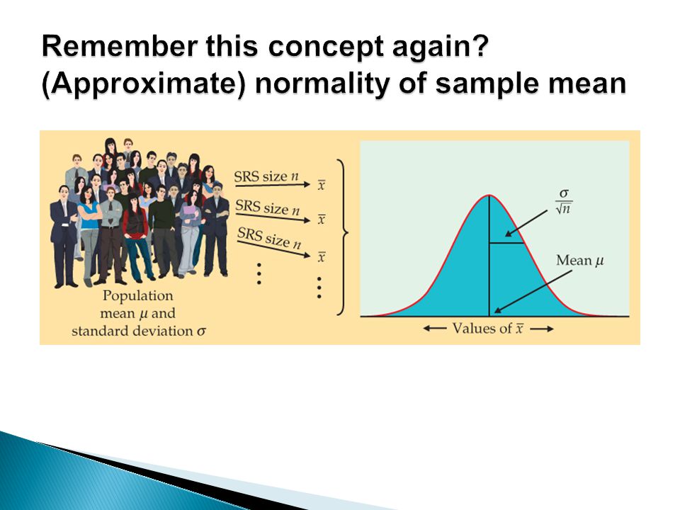
2. 2 Sampling Distributions The law of large numbers assures us that if we measure enough subjects, the statistic x-bar will eventually get very close to the unknown parameter µ. If we took every one of the possible samples of a certain size, calculated the sample mean for each, and graphed all of those values, we’d have a sampling distribution. The population distribution of a variable is the distribution of values of the variable among all individuals in the population. The sampling distribution of a statistic is the distribution of values taken by the statistic in all possible samples of the same size from the same population. The population distribution of a variable is the distribution of values of the variable among all individuals in the population. The sampling distribution of a statistic is the distribution of values taken by the statistic in all possible samples of the same size from the same population.

3.  Example: ◦ n = 2500 adults asked whether shopping is frustrating  n is the number of trials ◦ X = 1650 answered “ Yes ”  X is the number of “successes” ◦ p-hat = X/n = 0.66 is the sample proportion (of successes)  Need to make sure we distinguish between the count and the sample proportion

4. 1.Each observation falls in just two categories:  Success/Failure  Heads/Tails  Yes/No 2.All observations are independent 3.Fixed number of trials, n 4.The probability of success, p, is the same in each trial  The distribution of the (total) count of successes in this binomial setting is: Binomial distribution denoted B(n,p)

5.  Toss a fair coin 10 times and count the number X of heads ◦ Binomial or not? ◦ What about a biased coin?  Deal 10 cards from a shuffled deck of 52. X is the number of spades. ◦ Binomial? ◦ Suggestions?  Number of girls born among first 100 children in a (large) hospital this year  Number of girls born in this hospital so far this year

6.  SRS is not quite a Binomial setting ◦ Why? Check the 4 properties!  However, if the population is 10 times larger than our sample n, then the number of “ successes ” in the sample is approximately Binomial. ◦ We say B(n,p) ◦ Here p is the population success rate  usually unknown

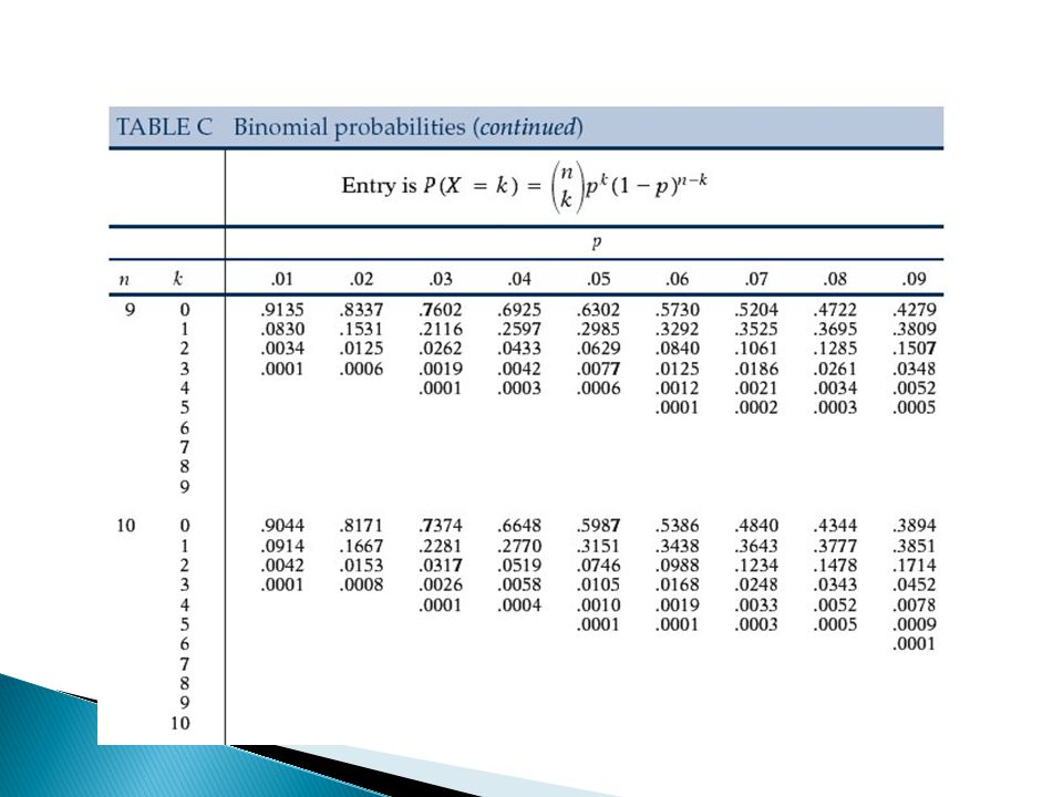
7.  We will just use table C  For given n and p, table gives the probability for k successes  Table only gives p ’ s of 0.5 or less ◦ If you have a p greater than 0.5, you need to switch the role of successes and failures.

12.  Bill is the star player on his basketball team. Over his career, his free throw percentage is 75%. However, his three-point shot percentage is only 20%. ◦ If he tries 5 three-point shots, what is the probability he will make 2? ◦ If he tries 10 free throws, what is the probability he will make 7? ◦ If he tries 10 free throws again, what is the probability he makes at least 7 free throws?

14.  Need to create a dataset with variable names for the probabilities you want  For example, probbnml(p,n,k) will give you the probability less than or equal to k successes. This is considered a variable, we need to name it, such as … prob_less_than_or_equal_to_k = probbnml(p,n,k);  What if we want greater than? prob_greater_than = 1 – probbnml(p,n,k);  What if we want equal to? prob_equal = probbnml(p,n,k) – probbnml(p,n,k-1);

15.  Calculate probabilities for binomial distribution: B(n,p) data binomial; p=0.25; n=10; k=4; prob_less_than_or_equal_to_k = probbnml(p,n,k); prob_greater_than = 1 - probbnml(p,n,k); prob_equal = probbnml(p,n,k) - probbnml(p,n,k-1); run; proc print data=binomial; run;

16. Binomial Example prob_less_ prob_ than_or_ greater_ prob_ Obs p n k equal_to_k than equal 1 0.25 10 4 0.92187 0.078127 0.14600

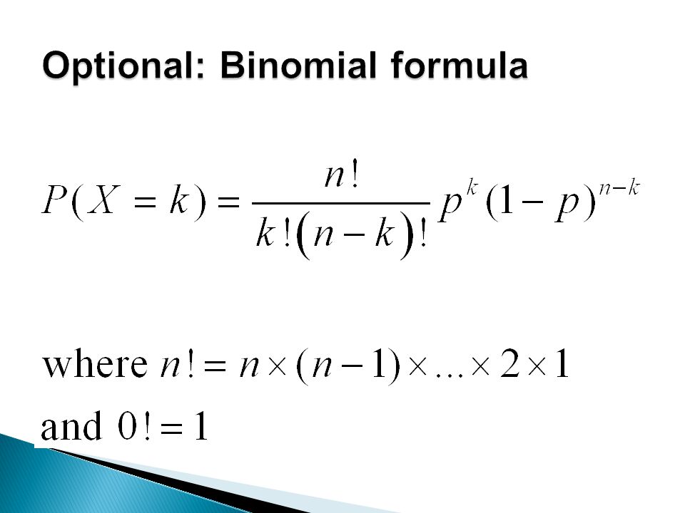
17.  If X has binomial distribution B(n,p) then

18.  For 10 tosses of a fair coin, let X = number of heads ◦ What is the distribution of X? ◦ Mean of X = ◦ Standard Deviation of X =

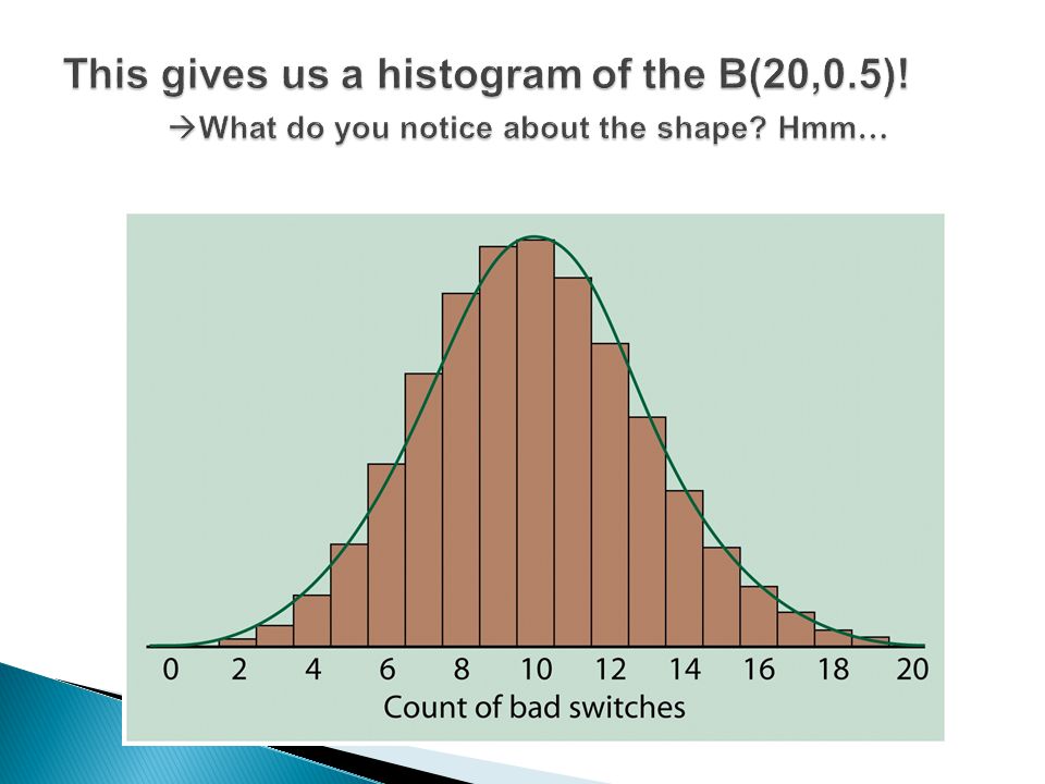
19.  Let us take a binomial situation … ◦ We have many bags with 20 switches in each bag ◦ The probability that each individual switch is bad is 0.5  So, the number of bad switches in each bag is a Binomial distribution with n = 20 and p = 0.5 ◦ B(20,0.5)  What if we look at how many switches are bad in many different bags?...draw a histogram!

21. 21 Normal Approximation for Binomial Distributions As n gets larger, something interesting happens to the shape of a binomial distribution. Suppose that X has the binomial distribution with n trials and success probability p. When n is large, the distribution of X is approximately Normal with mean and standard deviation As a rule of thumb, we will use the Normal approximation when n is so large that np ≥ 10 and n(1 – p) ≥ 10. Suppose that X has the binomial distribution with n trials and success probability p. When n is large, the distribution of X is approximately Normal with mean and standard deviation As a rule of thumb, we will use the Normal approximation when n is so large that np ≥ 10 and n(1 – p) ≥ 10. Normal Approximation for Binomial Distributions

22.  The sample proportion relates directly to the count X:  Counts or X:  Propotions or p-hat:

24.  In 2001, Barry Bonds hit 73 home runs. Was this feat as surprising as most of us thought? In the prior two seasons, Bonds hit a home run in 10% of his times at bat. If he went to bat 476 times in 2001, what is the probability that he hits 73 or more home runs just by chance? (Solve in terms of both X and p-hat.) Is it appropriate to use the normal approximation for this problem?  (The real probability from the Binomial is 0.0001)

25.  What is the probability that the percentage of heads in 100 tosses is between 40% and 60%?  Assume that exactly 60% of population does not like shopping. What is the chance of obtaining sample proportion larger than 0.65 for sample size=2500?

26.  Sampling distribution of sample counts and proportions  Evaluating the Binomial Probabilities  Using the approximate sample distribution to assess certain probabilities  The probabilities evaluated using the normal distribution are not exact, but approximations

27.  Population distribution vs. sampling distribution  The mean and standard deviation of the sample mean  Sampling distribution of a sample mean  Central limit theorem 27

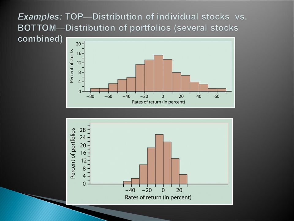
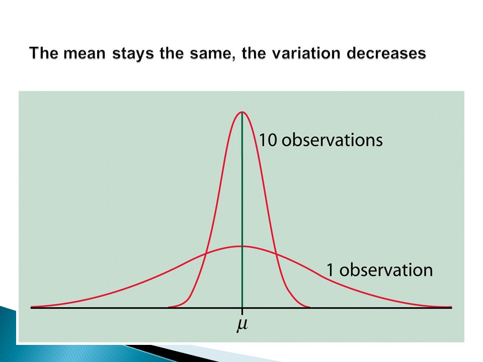
29.  Because portfolios usually contain many individual stocks, when we look at the return of portfolios, we are looking at the return of the sum (or average) of many individual stocks  What happens to the distribution of the portfolios?  Let ’ s look again …

30.  Given an SRS of size n, we observe n values X 1, X 2,…, X n, of a quantitative random variable  The sample mean of the SRS is:

31.  Assume the population has mean µ and standard deviation σ.  Then if the observations are independent, the sample mean, x_bar, has population mean and standard deviation given as follows:

32.  The height in inches of a randomly chosen young woman is N(64.5, 2.5)  What is the mean and standard deviation of the average of 100 randomly chosen young women? ◦ Think in terms of stocks and portfolios ◦ What will the normal distribution above do?

34.  If the variable X in the population is N(µ,σ) then  Kicker: This is often a good approximation even if the original distribution is not normal.  This is a HUGE result, called the Central Limit Theorem (or CLT).  It says if we start with ANY distribution, the sample mean will be normally distributed.

35.  Take 100 randomly chosen young women and measure their height. What is the chance that the average height of these 100 women is between 64 and 65 inches?

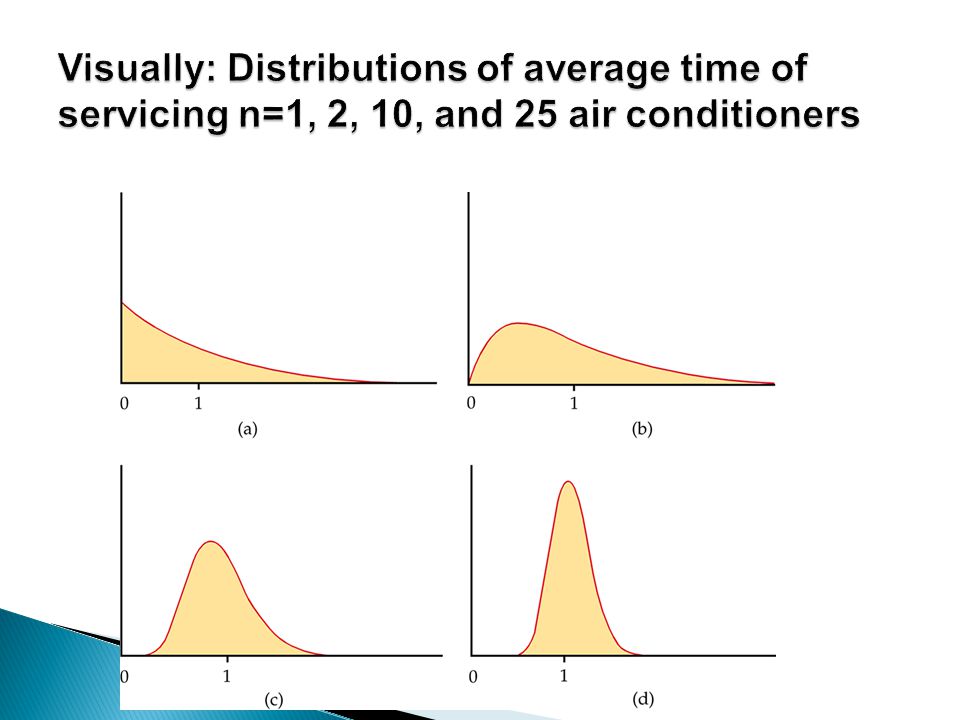
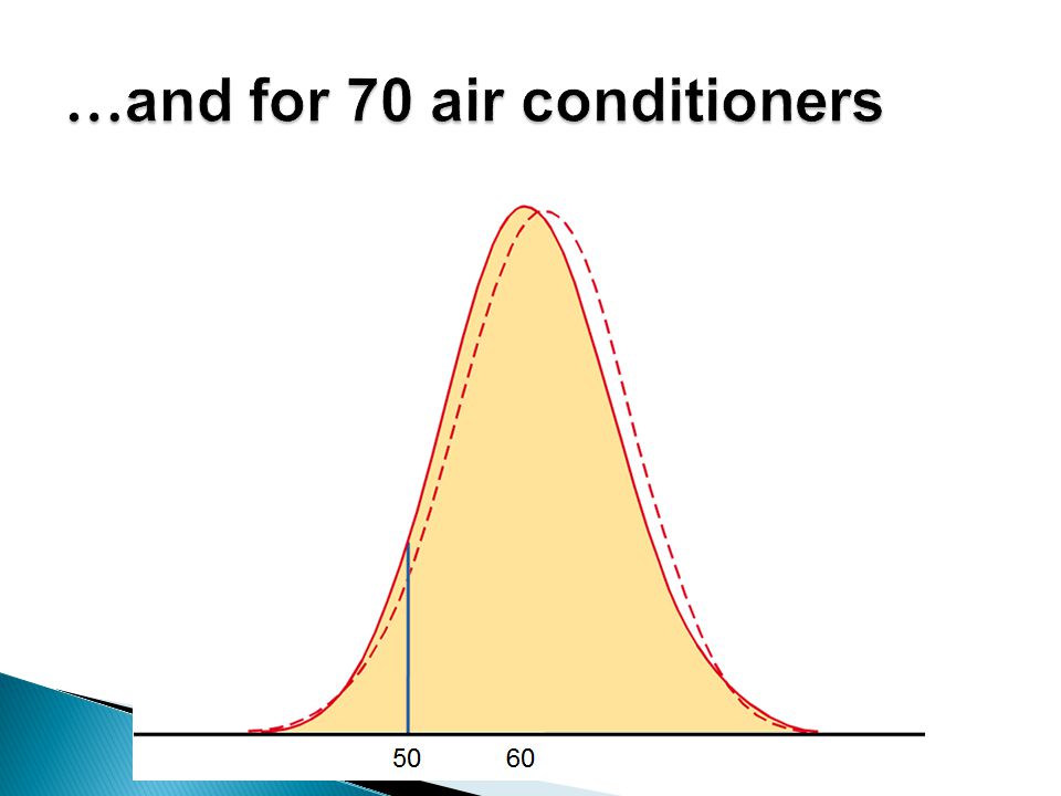
36.  The mean time for maintenance of an air conditioner is 60 minutes, with a standard deviation of 60 minutes.  What is the probability that average maintenance time of 70 air conditioners will exceed 50 minutes? ◦ Note, we didn ’ t say the time for maintenance is normally distributed. In fact, it follows an exponential distribution.

40.  If you know n, then the distributions for the sum and average are equivalent (if you know one, you know the other). ◦ So since has a normal distribution, then sums are also normally distributed!  A count (think binomial) is just a sum! ◦ We are just adding up individual observations, of course that is a sum and hence normal! ◦ So of course counts are normal! ◦ Similarly proportions function like averages, and are also normally distributed!  The CLT is the key.

41.  This is our (familiar) approximate normality.  Important assumptions: ◦ SRS (Simple Random Sample) ◦ Population distribution of X has mean µ and standard deviation σ; ◦ Last but not least, n needs to be “large enough”. Remember the air conditioning example. Generally, we say n ≥ 30 is “large enough”.  Warning: not all interesting distributions are normal ◦ But, the sample means are always roughly normal for large sample sizes.

42.  Approximate normal distribution of the sample mean from a SRS.  CLT holds for ANY population distribution.  Also, if in fact the underlying population distribution is exact (in some cases it is), then the result is also exact, not an approximation.  Use the CLT to evaluate probabilities regarding averages.

43.  How do you tell the “ X-bar ” problems apart from section 1.3 “ X ” problems? ◦ Section 1.3 “ X ” problems have a sample size of 1 (n = 1). ◦ Section 5.2 “ X-bar ” problems have a sample size bigger than 1.

44.  We flip cards from a stack of cards containing 10 normal decks of cards and count each time we flip an “ Ace ” as a success. ◦ What is the population proportion of success? ◦ If we only did 50 cards as a sample, and 4 aces were flipped, what is the sample proportion of success? ◦ If we did repeated samples of size n = 50, what is the mean and standard deviation of the sample proportion?

45.  Bob is playing in the club golf tournament. Bob ’ s scores vary as he plays the course repeatedly and has a N(77,3) distribution. ◦ What is the probability that Bob will shoot a 74 or lower in the first round of the club tournament? ◦ What is the probability that Bob will average 74 or lower for the 4 rounds of the club tournament?