1. Clustering Dr. Jieh-Shan George YEH jsyeh@pu.edu.tw

2. k-Means Clustering k-means clustering aims to partition n observations into k clusters in which each observation belongs to the cluster with the nearest mean, serving as a prototype of the cluster. The problem is computationally difficult (NP- hard)

3. k-Means Clustering: Example iris2 <- iris # remove species from the data iris2$Species <- NULL # the cluster number is set to 3 kmeans.result <- kmeans(iris2, 3) table(iris$Species, kmeans.result$cluster)

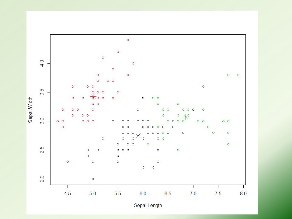
4. plot(iris2[c("Sepal.Length", "Sepal.Width")], col = kmeans.result$cluster) # plot cluster centers points(kmeans.result$centers[,c("Sepal.Length", "Sepal.Width")], col = 1:3, pch = 8, cex=2)

6. FPC: FLEXIBLE PROCEDURES FOR CLUSTERING http://cran.r-project.org/web/packages/fpc/index.html

7. k-Medoids Clustering The k-medoids algorithm is a clustering algorithm k-medoids chooses datapoints as centers (medoids or exemplars) The most common realization of k-medoid clustering is the Partitioning Around Medoids (PAM) algorithm

8. k-Medoids Clustering #PAM (Partitioning Around Medoids) library(fpc) pamk.result <- pamk(iris2) # number of clusters pamk.result$nc # check clustering against actual species table(pamk.result$pamobject$clustering, iris$Species)

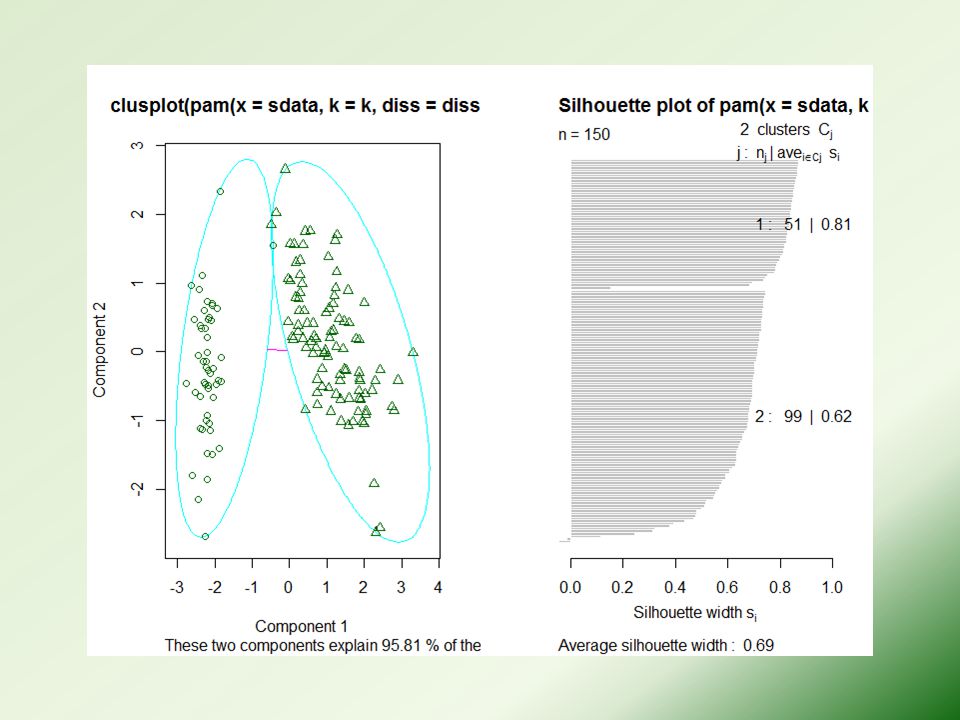
9. layout(matrix(c(1,2),1,2)) # 2 graphs per page plot(pamk.result$pamobject) layout(matrix(1)) # change back to one graph per page # pamk() produces two clusters: one is "setosa", and the other is a mixture of "versicolor" and "virginica".

11. CLUSTER: CLUSTER ANALYSIS EXTENDED ROUSSEEUW ET AL http://cran.r-project.org/web/packages/cluster/index.html

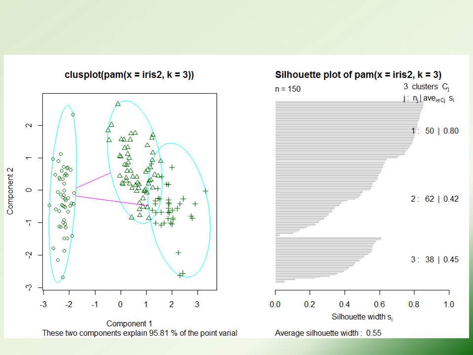
12. Partitioning Around Medoids (PAM) library(cluster) pam.result <- pam(iris2, 3) table(pam.result$clustering, iris$Species) layout(matrix(c(1,2),1,2)) # 2 graphs per page plot(pam.result) layout(matrix(1)) # change back to one graph per page

14. It's hard to say which one is better out of the above two clusterings produced respectively with pamk() and pam(). It depends on the target problem and domain knowledge and experience. In

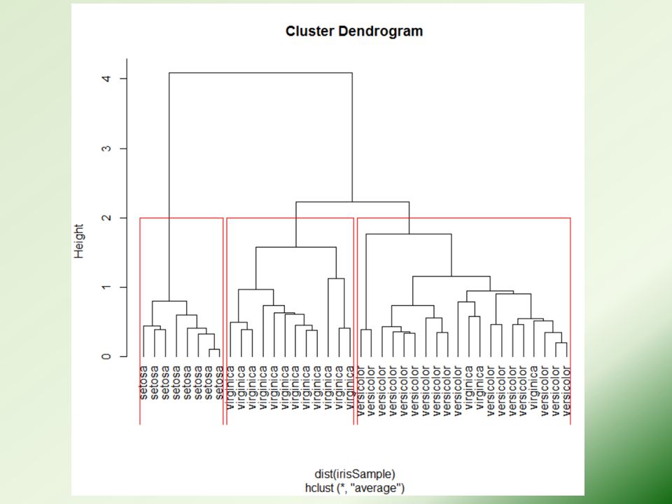
15. Hierarchical Clustering # sample of 40 records from the iris data, so that the clustering plot will not be over crowded. idx <- sample(1:dim(iris)[1], 40) irisSample <- iris[idx,] irisSample$Species <- NULL hc <- hclust(dist(irisSample), method="ave") plot(hc, hang = -1, labels=iris$Species[idx]) # cut tree into 3 clusters rect.hclust(hc, k=3) groups <- cutree(hc, k=3)

17. Density-based Clustering DBSCAN density reachability and connectivity clustering library(fpc) iris2 <- iris[-5] # remove class tags ds <- dbscan(iris2, eps=0.42, MinPts=5)

18. # compare clusters with original class labels table(ds$cluster, iris$Species) "1" to "3" in the first column are three identified clusters, while " 0" stands for noises or outliers

19. plot(ds, iris2)

20. plot(ds, iris2[c(1,4)])

21. plotcluster(iris2, ds$cluster)

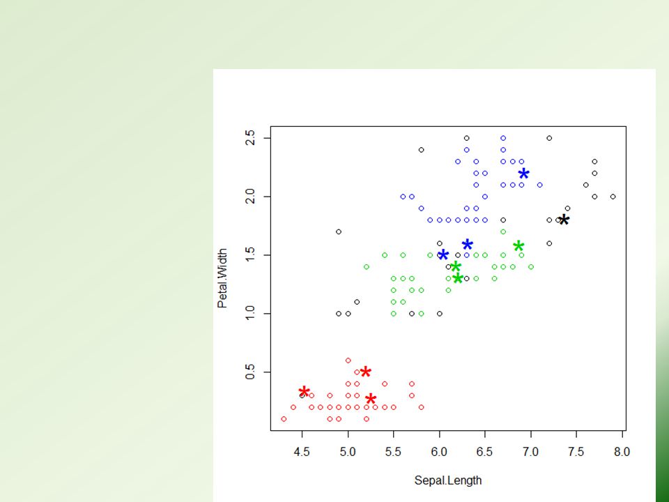
22. label new data # create a new dataset for labeling set.seed(435) idx <- sample(1:nrow(iris), 10) newData <- iris[idx,-5] newData <- newData + matrix(runif(10*4, min=0, max=0.2), nrow=10, ncol=4) # label new data myPred <- predict(ds, iris2, newData) # plot result plot(iris2[c(1,4)], col=1+ds$cluster) points(newData[c(1,4)], pch="*", col=1+myPred, cex=3) # check cluster labels table(myPred, iris$Species[idx])