Download presentation
Presentation is loading. Please wait.

1
Chapter 2 Simple Comparative Experiments

2
2.1 Introduction Consider experiments to compare two conditions
Simple comparative experiments Example: The strength of portland cement mortar Two different formulations: modified v.s. unmodified Collect 10 observations for each formulations Formulations = Treatments (levels)
")
3
The data (Table 2.1) Observation (sample), j Modified Mortar
(Formulation 1) Unmodified Mortar (Formulation 2) 1 16.85 17.50 2 16.40 17.63 3 17.21 18.25 4 16.35 18.00 5 16.52 17.86 6 17.04 17.75 7 16.96 18.22 8 17.15 17.90 9 16.59 17.96 10 16.57 18.15
 Unmodified Mortar (Formulation 2)")
4
Dot diagram: Form 1 (modified) v.s. Form 2 (unmodified)
unmodified (17.92) > modified (16.76)
 > modified (16.76)")
5
Hypothesis testing (significance testing): a technique to assist the experiment in comparing these two formulations.
: a technique to assist the experiment in comparing these two formulations.")
6
2.2 Basic Statistical Concepts
Run = each observations in the experiment Error = random variable Graphical Description of Variability Dot diagram: the general location or central tendency of observations Histogram: central tendency, spread and general shape of the distribution of the data (Fig. 2-2)
")
7
Box-plot: minimum, maximum, the lower and upper quartiles and the median

8
Probability Distributions
Mean, Variance and Expected Values

9
2.3 Sampling and Sampling Distribution
Random sampling Statistic: any function of the observations in a sample that does not contain unknown parameters Sample mean and sample variance Properties of sample mean and sample variance Estimator and estimate Unbiased and minimum variance

10
Degree of freedom: Random variable y has v degree of freedom if E(SS/v) = σ2 The number of independent elements in the sum of squares The normal and other sampling distribution: Sampling distribution Normal distribution: The Central Limit Theorem Chi-square distribution: the distribution of SS t distribution F distribution

11
2.4 Inferences about the Differences in Means, Randomized Designs
Use hypothesis testing and confidence interval procedures for comparing two treatment means. Assume a completely randomized experimental design is used. (a random sample from a normal distribution)
")
12
2.4.1 Hypothesis Testing Compare the strength of two different formulations: unmodified v.s. modified Two levels of the factor yij : the the jth observation from the ith factor level, i=1, 2, and j = 1,2,…, ni

13
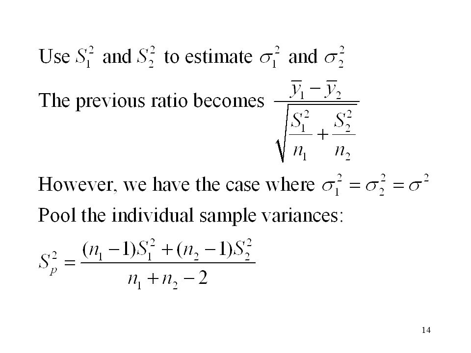
Model: yij = μi + ε ij yij ~ N( μ i, σi2) Statistical hypotheses: Test statistic, critical region (rejection region) Type I error, Type II error and Power The two-sample t-test:

15
Values of t0 that are near zero are consistent with the null hypothesis
Values of t0 that are very different from zero are consistent with the alternative hypothesis t0 is a “distance” measure-how far apart the averages are expressed in standard deviation units Notice the interpretation of t0 as a signal-to-noise ratio

17
So far, we haven’t really done any “statistics”
We need an objective basis for deciding how large the test statistic t0 really is In 1908, W. S. Gosset derived the reference distribution for t0 … called the t distribution Tables of the t distribution - text, page 640

18
A value of t0 between –2. 101 and 2
A value of t0 between –2.101 and is consistent with equality of means It is possible for the means to be equal and t0 to exceed either or –2.101, but it would be a “rare event” … leads to the conclusion that the means are different Could also use the P-value approach

19
The P-value is the risk of wrongly rejecting the null hypothesis of equal means (it measures rareness of the event) The P-value in our problem is P = 3.68E-8

20
Checking Assumptions in the t-test:
Equal-variance assumption Normality assumption Normal Probability Plot: y(j) v.s. (j – 0.5)/n
 v.s. (j – 0.5)/n.")
21
Estimate mean and variance from normal probability plot:
Mean: 50 percentile Variance: the difference between 84th and 50th percentile Transformations

22
2.4.2 Choice of Sample Size Type II error in the hypothesis testing Operating Characteristic curve (O.C. curve) Assume two population have the same variance (unknown) and sample size. For a specified sample size and , larger differences are more easily detected To detect a specified difference , the more powerful test, the more sample size we need.
 and sample size. For a specified sample size and , larger differences are more easily detected. To detect a specified difference , the more powerful test, the more sample size we need.")
23
2.4.3 Confidence Intervals The confidence interval on the difference in means General form of a confidence interval: The 100(1-) percent confidence interval on the difference in two means
 percent confidence interval on the difference in two means.")
24
2.5 Inferences about the Differences in Means, Paired Comparison Designs
Example: Two different tips for a hardness testing machine 20 metal specimens Completely randomized design (10 for tip 1 and 10 for tip 2) Lack of homogeneity between specimens An alternative experiment design: 10 specimens and divide each specimen into two parts.
 Lack of homogeneity between specimens. An alternative experiment design: 10 specimens and divide each specimen into two parts.")
25
The statistical model:
μ i is the true mean hardness of the ith tip, β j is an effect due to the jth specimen, ε ij is a random error with mean zero and variance σi2 The difference in the jth specimen: The expected value of this difference is

26
Testing μ 1 = μ 2 <=> testing μd = 0
The test statistic for H0: μd = 0 v.s. H1: μd ≠ 0 Under H0, t0 ~ tn-1 (paired t-test) Paired comparison design Block (the metal specimens) Several points: Only n-1 degree of freedom (2n observations) Reduce the variance and narrow the C.I. (the noise reduction property of blocking)
 Paired comparison design. Block (the metal specimens) Several points: Only n-1 degree of freedom (2n observations) Reduce the variance and narrow the C.I. (the noise reduction property of blocking)")
27
2.6 Inferences about the Variances of Normal Distributions
Test the variances Normal distribution Hypothesis: H0: σ 2 = σ02 v.s. H1: σ 2 ≠ σ02 The test statistic is Under H0, The 100(1-) C.I.:
 C.I.:")
28
Hypothesis: H0: σ12 = σ22 v.s. H1: σ12 ≠ σ22
The test statistic is F0 = S12/ S22 , and under H0, F0 = S12/ S22 ~ Fn1-1,n2-1 The 100(1-) C.I.:
 C.I.:")
Similar presentations

 2004 Brooks/Cole, a division of Thomson Learning, Inc. Chapter 9 Inferences Based on Two Samples.>")


