1. ONLINE Q-LEARNER USING MOVING PROTOTYPES by Miguel Ángel Soto Santibáñez

2. Reinforcement Learning What does it do? Tackles the problem of learning control strategies for autonomous agents. What is the goal? The goal of the agent is to learn an action policy that maximizes the total reward it will receive from any starting state.

3. Reinforcement Learning What does it need? This method assumes that training information is available in the form of a real-valued reward signal given for each state- action transition. This method assumes that training information is available in the form of a real-valued reward signal given for each state- action transition. i.e. (s, a, r) i.e. (s, a, r) What problems? Very often, reinforcement learning fits a problem setting known as a Markov decision process (MDP).

4. Reinforcement Learning vs. Dynamic programming reward function r(s, a)  r r(s, a)  r state transition function state transition function δ(s, a)  s’ δ(s, a)  s’

5. Q-learning An off-policy control algorithm. Advantage: Converges to an optimal policy in both deterministic and nondeterministic MDPs. Disadvantage: Only practical on a small number of problems.

6. Q-learning Algorithm Initialize Q(s, a) arbitrarily Repeat (for each episode) Repeat (for each episode) Initialize s Initialize s Repeat (for each step of the episode) Repeat (for each step of the episode) Choose a from s using an exploratory policy Choose a from s using an exploratory policy Take action a, observe r, s’ Take action a, observe r, s’ Q(s, a)  Q(s, a) + α[r + γ max Q(s’, a’) – Q(s, a)] Q(s, a)  Q(s, a) + α[r + γ max Q(s’, a’) – Q(s, a)] a’ a’ s  s’ s  s’

7. Introduction to Q-learning Algorithm An episode: { (s 1, a 1, r 1 ), (s 2, a 2, r 2 ), … (s n, a n, r n ), } An episode: { (s 1, a 1, r 1 ), (s 2, a 2, r 2 ), … (s n, a n, r n ), } s’: δ(s, a)  s’ s’: δ(s, a)  s’ Q(s, a): Q(s, a): γ, α : γ, α :

8. A Sample Problem A B r = 8 r = 0 r = - 8

9. States and actions 12345 678910 1112131415 1617181920 states:actions: NSEWNSEW

10. The Q(s, a) function 1234567891011121314151617181920 N S W E states actionsactions

11. Q-learning Algorithm Initialize Q(s, a) arbitrarily Repeat (for each episode) Repeat (for each episode) Initialize s Initialize s Repeat (for each step of the episode) Repeat (for each step of the episode) Choose a from s using an exploratory policy Choose a from s using an exploratory policy Take action a, observe r, s’ Take action a, observe r, s’ Q(s, a)  Q(s, a) + α[r + γ max Q(s’, a’) – Q(s, a)] Q(s, a)  Q(s, a) + α[r + γ max Q(s’, a’) – Q(s, a)] a’ a’ s  s’ s  s’

12. Initializing the Q(s, a) function 1234567891011121314151617181920 N00000000000000000000 S00000000000000000000 W00000000000000000000 E00000000000000000000 states actionsactions

13. Q-learning Algorithm Initialize Q(s, a) arbitrarily Repeat (for each episode) Repeat (for each episode) Initialize s Initialize s Repeat (for each step of the episode) Repeat (for each step of the episode) Choose a from s using an exploratory policy Choose a from s using an exploratory policy Take action a, observe r, s’ Take action a, observe r, s’ Q(s, a)  Q(s, a) + α[r + γ max Q(s’, a’) – Q(s, a)] Q(s, a)  Q(s, a) + α[r + γ max Q(s’, a’) – Q(s, a)] a’ a’ s  s’ s  s’

14. An episode 12345 678910 1112131415 1617181920

15. Q-learning Algorithm Initialize Q(s, a) arbitrarily Repeat (for each episode) Repeat (for each episode) Initialize s Initialize s Repeat (for each step of the episode) Repeat (for each step of the episode) Choose a from s using an exploratory policy Choose a from s using an exploratory policy Take action a, observe r, s’ Take action a, observe r, s’ Q(s, a)  Q(s, a) + α[r + γ max Q(s’, a’) – Q(s, a)] Q(s, a)  Q(s, a) + α[r + γ max Q(s’, a’) – Q(s, a)] a’ a’ s  s’ s  s’

16. Calculating new Q(s, a) values 1 st step:2 nd step: 3 rd step: 4 th step:

17. The Q(s, a) function after the first episode 1234567891011121314151617181920 N000000-80000000000000 S00000000000000000000 W00000000000000000000 E00000000000000000000 states actionsactions

18. A second episode 12345 678910 1112131415 1617181920

19. Calculating new Q(s, a) values 1 st step:2 nd step: 3 rd step: 4 th step:

20. The Q(s, a) function after the second episode 1234567891011121314151617181920 N000000-80000000000000 S00000000000000000000 W00000000000000000000 E00000000800000000000 states actionsactions

21. The Q(s, a) function after a few episodes 1234567891011121314151617181920 N000000-8-8-800124000000 S0000000.51200-8-8-8000000 W000000-81200-80.51000000 E0000002480012-8000000 states actionsactions

22. One of the optimal policies 1234567891011121314151617181920 N000000-8-8-800124000000 S0000000.51200-8-8-8000000 W000000-81200-80.51000000 E0000002480012-8000000 states actionsactions

23. An optimal policy graphically 12345 678910 1112131415 1617181920

24. Another of the optimal policies 1234567891011121314151617181920 N000000-8-8-800124000000 S0000000.51200-8-8-8000000 W000000-81200-80.51000000 E0000002480012-8000000 states actionsactions

25. Another optimal policy graphically 12345 678910 1112131415 1617181920

26. The problem with tabular Q-learning What is the problem? Only practical in a small number of problems because: a)Q-learning can require many thousands of training iterations to converge in even modest-sized problems. b)Very often, the memory resources required by this method become too large.

27. Solution What can we do about it? Use generalization. Use generalization. What are some examples? Tile coding, Radial Basis Functions, Fuzzy function approximation, Hashing, Artificial Neural Networks, LSPI, Regression Trees, Kanerva coding, etc.

28. Shortcomings Tile coding: Curse of Dimensionality. Tile coding: Curse of Dimensionality. Kanerva coding: Static prototypes. Kanerva coding: Static prototypes. LSPI: Require a priori knowledge of the Q-function. LSPI: Require a priori knowledge of the Q-function. ANN: Require a large number of learning experiences. ANN: Require a large number of learning experiences. Batch + Regression trees: Slow and requires lots of memory. Batch + Regression trees: Slow and requires lots of memory.

29. Needed properties 1)Memory requirements should not explode exponentially with the dimensionality of the problem. 2)It should tackle the pitfalls caused by the usage of “static prototypes”. 3)It should try to reduce the number of learning experiences required to generate an acceptable policy. NOTE: All this without requiring a priori knowledge of the Q-function. NOTE: All this without requiring a priori knowledge of the Q-function.

30. Overview of the proposed method 1) The proposed method limits the number of prototypes available to describe the Q-function (as Kanerva coding). 2) The Q-function is modeled using a regression tree (as the batch method proposed by Sridharan and Tesauro). 3) But prototypes are not static, as in Kanerva coding, but dynamic. 4) The proposed method has the capacity to update the Q- function once for every available learning experience (it can be an online learner).

31. Changes on the normal regression tree

32. Basic operations in the regression tree Rupture Rupture Merging Merging

33. Impossible Merging

34. Rules for a sound tree parent children parent

35. Impossible Merging

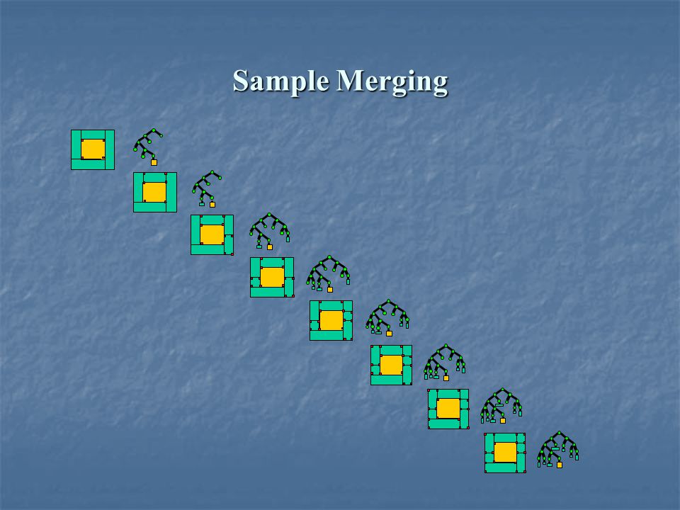
36. Sample Merging The “smallest predecessor”

37. Sample Merging List 1

38. Sample Merging The node to be inserted

39. Sample Merging List 1 List 1.1 List 1.2

40. Sample Merging

43. The agent Detectors’ Signals Actuators’ Signals Agent Reward

44. Applications BOOK STORE

45. Results first application TabularQ-learningMovingPrototypesBatchMethod PolicyQualityBestBestWorst ComputationalComplexity O(n) O(n log(n)) O(n2) O(n3) MemoryUsageBadBestWorst

46. Results first application (details) TabularQ-learningMovingPrototypesBatchMethod PolicyQuality $2,423,355$2,423,355$2,297,100 MemoryUsage10,202prototypes413prototypes11,975prototypes

47. Results second application MovingPrototypesLSPI(least-squares policy iteration) PolicyQualityBestWorst ComputationalComplexity O(n log(n)) O(n2) O(n) MemoryUsageWorstBest

48. Results second application (details) MovingPrototypesLSPI(least-squares policy iteration) PolicyQuality forever (succeeded) 26 time steps (failed) 170 time steps (failed) forever (succeeded) Required Learning Experiences 2163242161,902,621183,618648 MemoryUsage about 170 prototypes 2 weight parameters

49. Results third application Reason for this experiment: Evaluate the performance of the proposed method in a scenario that we consider ideal for this method, namely one, for which there is no application specific knowledge available. What took to learn a good policy: Less than 2 minutes of CPU time. Less than 2 minutes of CPU time. Less that 25,000 learning experiences. Less that 25,000 learning experiences. Less than 900 state-action-value tuples. Less than 900 state-action-value tuples.

50. Swimmer first movie

51. Swimmer second movie

52. Swimmer third movie

53. Future Work Different types of splits. Different types of splits. Continue characterization of the method Moving Prototypes. Continue characterization of the method Moving Prototypes. Moving prototypes + LSPI. Moving prototypes + LSPI. Moving prototypes + Eligibility traces. Moving prototypes + Eligibility traces.