Download presentation
Presentation is loading. Please wait.

1
10/22 Homework 3 returned; solutions posted Homework 4 socket opened Project 3 assigned Mid-term on Wednesday (Optional) Review session Tuesday
 Review session Tuesday")
2
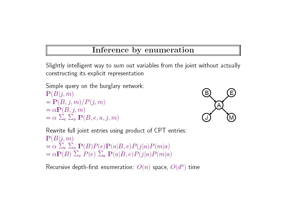
Conjunctive queries are essentially computing joint distributions on sets of query variables. A special case of computing the full joint on query variables is finding just the query variable configuration that is Most likely given the evidence. There are two special cases here Also MPE—Most Probable Explanation Most likely assignment to all other variables given the evidence Mostly involves max/product MAP—Maximum a posteriori Most likely assignment to some variables given the evidence Can involve, max/product/sum operations

3
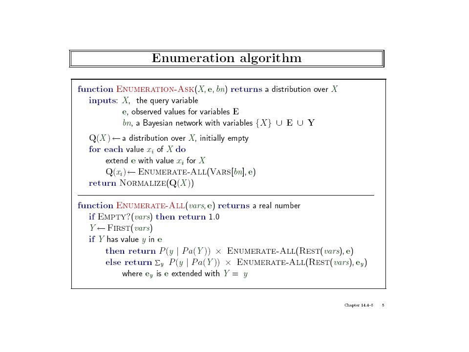
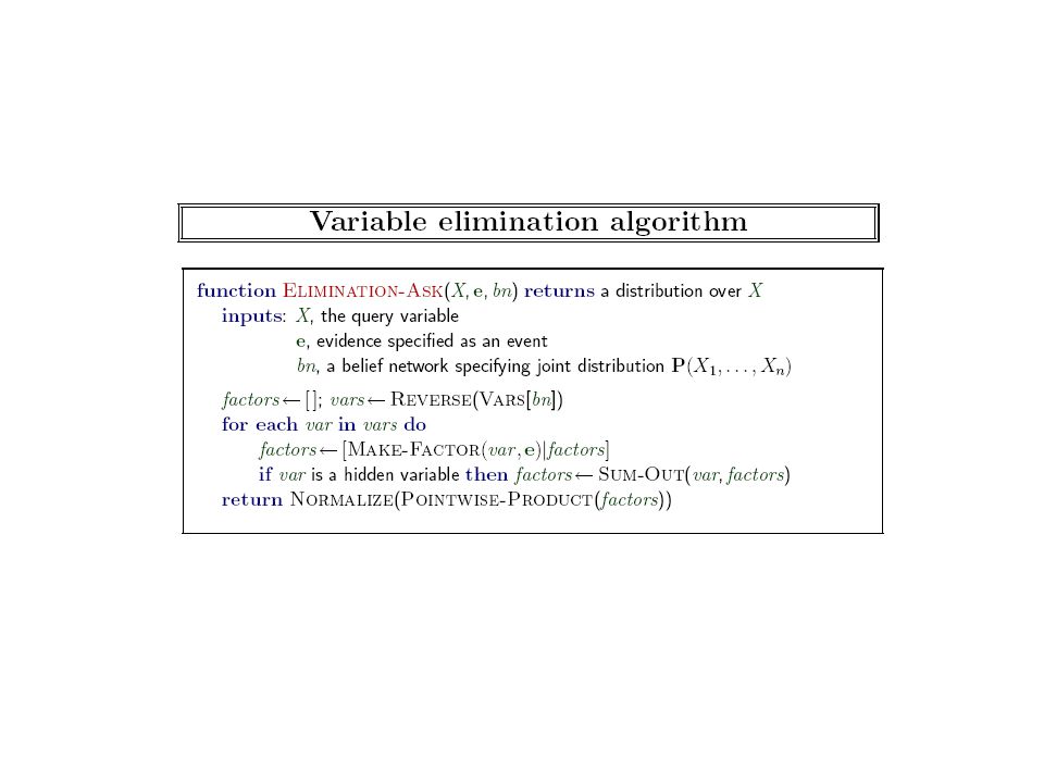
Overview of BN Inference Algorithms Exact Inference Complexity –NP-hard (actually #P-Complete; since we “count” models) Polynomial for “Singly connected” networks (one path between each pair of nodes) Algorithms –Enumeration –Variable elimination Avoids the redundant computations of Enumeration –[Many others such as “message passing” algorithms, Constraint- propagation based algorithms etc.] Approximate Inference Complexity –NP-Hard for both absolute and relative approximation Algorithms –Based on Stochastic Simulation Sampling from empty networks Rejection sampling Likelihood weighting MCMC [And many more] TONS OF APPROACHES
![Overview of BN Inference Algorithms Exact Inference Complexity –NP-hard (actually #P-Complete; since we count models) Polynomial for Singly connected networks (one path between each pair of nodes) Algorithms –Enumeration –Variable elimination Avoids the redundant computations of Enumeration –[Many others such as message passing algorithms, Constraint- propagation based algorithms etc.] Approximate Inference Complexity –NP-Hard for both absolute and relative approximation Algorithms –Based on Stochastic Simulation Sampling from empty networks Rejection sampling Likelihood weighting MCMC [And many more] TONS OF APPROACHES](http://images.slideplayer.com/16/5229670/slides/slide_3.jpg "Overview of BN Inference Algorithms Exact Inference Complexity –NP-hard (actually #P-Complete; since we count models) Polynomial for Singly connected networks (one path between each pair of nodes) Algorithms –Enumeration –Variable elimination Avoids the redundant computations of Enumeration –[Many others such as message passing algorithms, Constraint- propagation based algorithms etc.] Approximate Inference Complexity –NP-Hard for both absolute and relative approximation Algorithms –Based on Stochastic Simulation Sampling from empty networks Rejection sampling Likelihood weighting MCMC [And many more] TONS OF APPROACHES")
4
Network Topology & Complexity of Inference Singly Connected Networks (poly-trees – At most one path between any pair of nodes) Inference is polynomial Cloudy Sprinklers Rain Wetgrass Multiply- connected Inference NP-hard Can be converted to singly-connected (by merging nodes) Cloudy Wetgrass Sprinklers+Rain (takes 4 values 2x2) The “size” of the merged network can beExponentially larger (so polynomial inferenceOn that network isn’t exactly god’s gift
 Inference is polynomial Cloudy Sprinklers Rain Wetgrass Multiply- connected Inference NP-hard Can be converted to singly-connected (by merging nodes) Cloudy Wetgrass Sprinklers+Rain (takes 4 values 2x2) The size of the merged network can beExponentially larger (so polynomial inferenceOn that network isn’t exactly god’s gift ")
5
Examples of singly connected networks include Markov Chains and Hidden Markov Models

9
f A (a,b,e)*f j (a)*f M (a)+ f A (~a,b,e)*f j (~a)*f M (~a)+
*f j (a)*f M (a)+ f A (~a,b,e)*f j (~a)*f M (~a)+")
10
Complexity depends on the size of the largest factor which in turn depends on the order in which variables are eliminated..

12
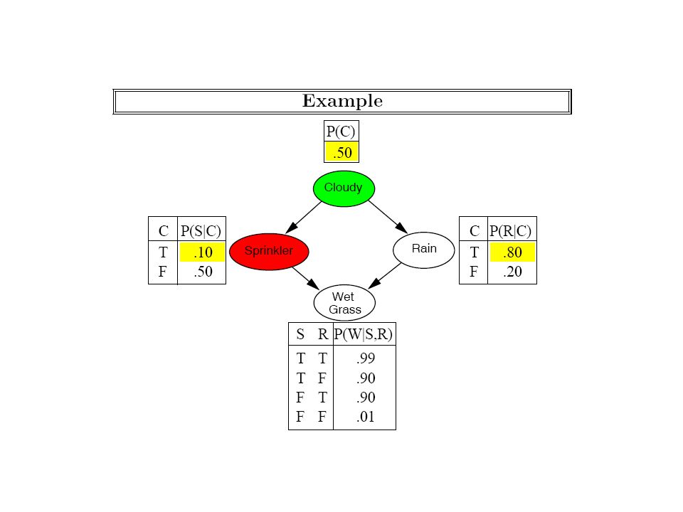
Variable Elimination and Irrelevant Variables… Suppose we asked the query P(J|A=t) –Which is probability that John calls given that Alarm went off –We know that this is a simple lookup into the CPT in our bayes net. –But, variable elimination algorithm is going to sum over the three other variables unnecessarily –In those cases, the factors will be “degenerate” (will sum to 1; see next slide) This problem can be even more prominent if we had many other variables in the network Qn: How can we make variable elimination wake-up and avoid this unnecessary work? –General answer is to (a) identify variables that are irrelevant given the query and evidence –In the P(J|A), we should be able to see that e,b,m are irrelevant and remove them (b) remove the irrelevant variables from the network –A variable v is irrelevant for a query P(X|E) if X || v | E (i.e., X is conditionally independent of v given E). We can use BayesBall or DSEP notions to figure out irrelevant variables v There are a couple of easier sufficient conditions for irrelevance (both of which are special cases of BayesBall/DSep).
 This problem can be even more prominent if we had many other variables in the network Qn: How can we make variable elimination wake-up and avoid this unnecessary work. –General answer is to (a) identify variables that are irrelevant given the query and evidence –In the P(J|A), we should be able to see that e,b,m are irrelevant and remove them (b) remove the irrelevant variables from the network –A variable v is irrelevant for a query P(X|E) if X || v | E (i.e., X is conditionally independent of v given E). We can use BayesBall or DSEP notions to figure out irrelevant variables v There are a couple of easier sufficient conditions for irrelevance (both of which are special cases of BayesBall/DSep)..")
13
In general, any leaf node that is not a query or evidence variable is irrelevant (and can be removed) (once it is removed, others may be seen to be irrelevant) Can drop irrelevant variables from the network before starting the query off.. Sufficient Condition 1

14
Sufficient Condition 2 Note that condition 2 doesn’t subsume condition 1. In particular, it won’t allow us to say that M is irrelevant for the query P(J|B)
.")
15
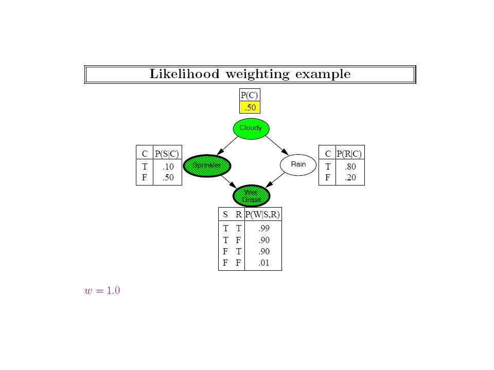
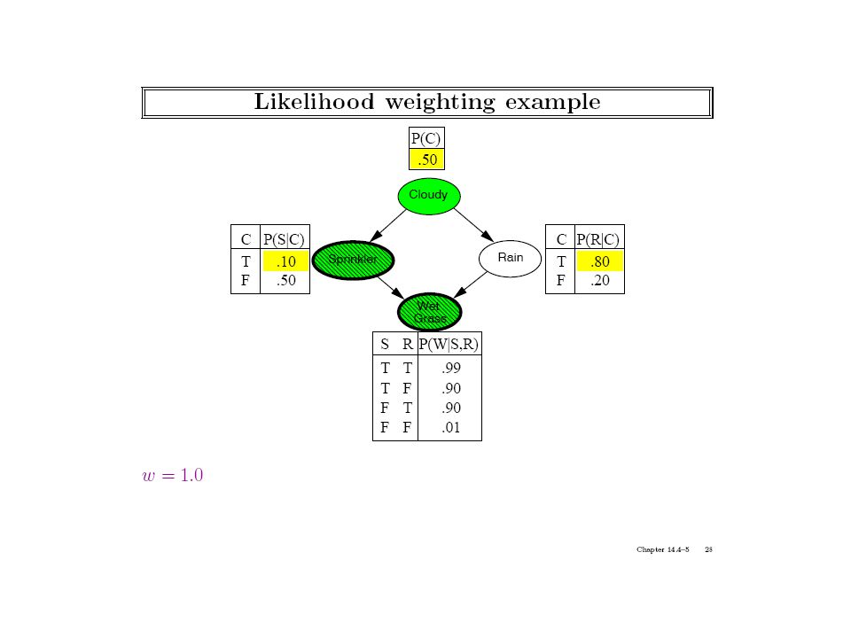
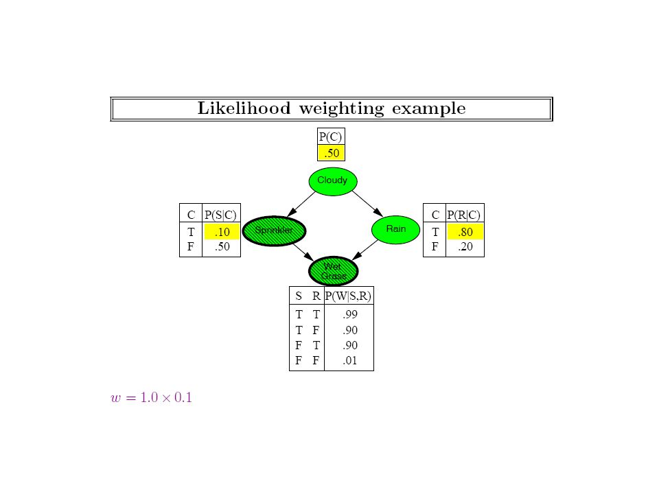
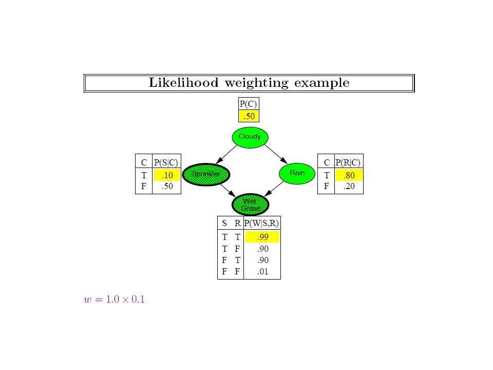
Notice that sampling methods could in general be used even when we don’t know the bayes net (and are just observing the world)! We should strive to make the sampling more efficient given that we know the bayes net

23
Generating a Sample from the Network Network Samples Joint distribution

25
That is, the rejection sampling method doesn’t really use the bayes network that much…

27
Notice that to attach the likelihood to the evidence, we are using the CPTs in the bayes net. (Model-free empirical observation, in contrast, either gives you a sample or not; we can’t get fractional samples)
.")
37
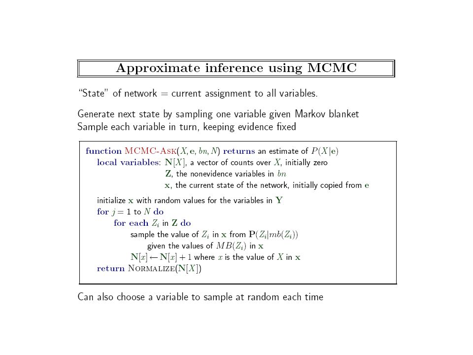
MCMC not covered

40
Note that the other parents of z j are part of the markov blanket

42
Case Study: Pathfinder System Domain: Lymph node diseases –Deals with 60 diseases and 100 disease findings Versions: –Pathfinder I: A rule-based system with logical reasoning –Pathfinder II: Tried a variety of approaches for uncertainity Simple bayes reasoning outperformed –Pathfinder III: Simple bayes reasoning, but reassessed probabilities –Parthfinder IV: Bayesian network was used to handle a variety of conditional dependencies. Deciding vocabulary: 8 hours Devising the topology of the network: 35 hours Assessing the (14,000) probabilities: 40 hours –Physician experts liked assessing causal probabilites Evaluation: 53 “referral” cases –Pathfinder III: 7.9/10 –Pathfinder IV: 8.9/10 [Saves one additional life in every 1000 cases!] –A more recent comparison shows that Pathfinder now outperforms experts who helped design it!!
 probabilities: 40 hours –Physician experts liked assessing causal probabilites Evaluation: 53 referral cases –Pathfinder III: 7.9/10 –Pathfinder IV: 8.9/10 [Saves one additional life in every 1000 cases!] –A more recent comparison shows that Pathfinder now outperforms experts who helped design it!!.")
Similar presentations


 (Slides from Sam Roweis)>")
>")


 Process A temporal process is the evolution of system state over time Often the system state.>")
>")

 Capturing uncertain knowledge Probabilistic.>")


 --Homework 3 due Thursday --Midterm next Thursday (10/26)>")
 = ?>")

